7 Beams
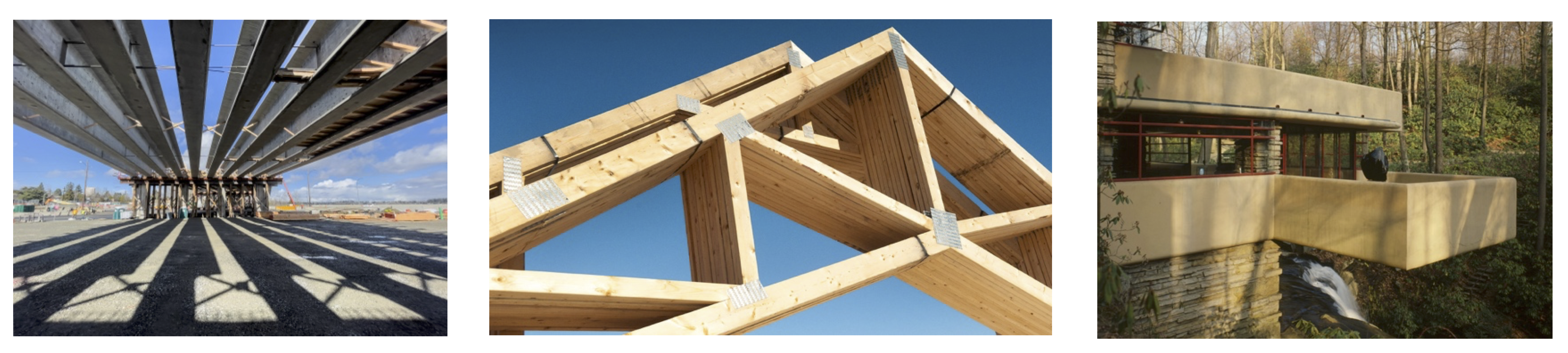
Beams are structural members that support loads along their length. Typically these loads are perpendicular to the axis of the beam and cause only shear and bending moments. Figure 7.1 shows some examples.
As evident in previous chapters, internal forces and moments are crucial to calculating stresses and deflections. The same is true for finding stresses and deflections in beams. Due to the nature of the loadings and constraints of beams, finding internal forces requires new methods in statics. This chapter describes these methods for finding a beam’s internal shear force and bending moments.
Section 7.1 reviews how to find the internal shear force and bending moments at a specific point in a beam using equilibrium. Section 7.2 discusses relationships between the applied load, the internal shear force, and the internal bending moment.
Then follows a discussion of a more general approach to visualizing the internal shear force and bending moment at different points in a beam using diagrams of these. Section 7.3 explores how to draw these diagrams using an equilibrium method. Then Section 7.4 provides an alternative graphical method for drawing these diagrams.
Before presenting methods for finding internal shear and moments of beams, we need to establish a sign convention to provide consistency and act as a guide to interpreting our results. Note that anytime you start a new project or subject, you should ensure that a sign convention is established.
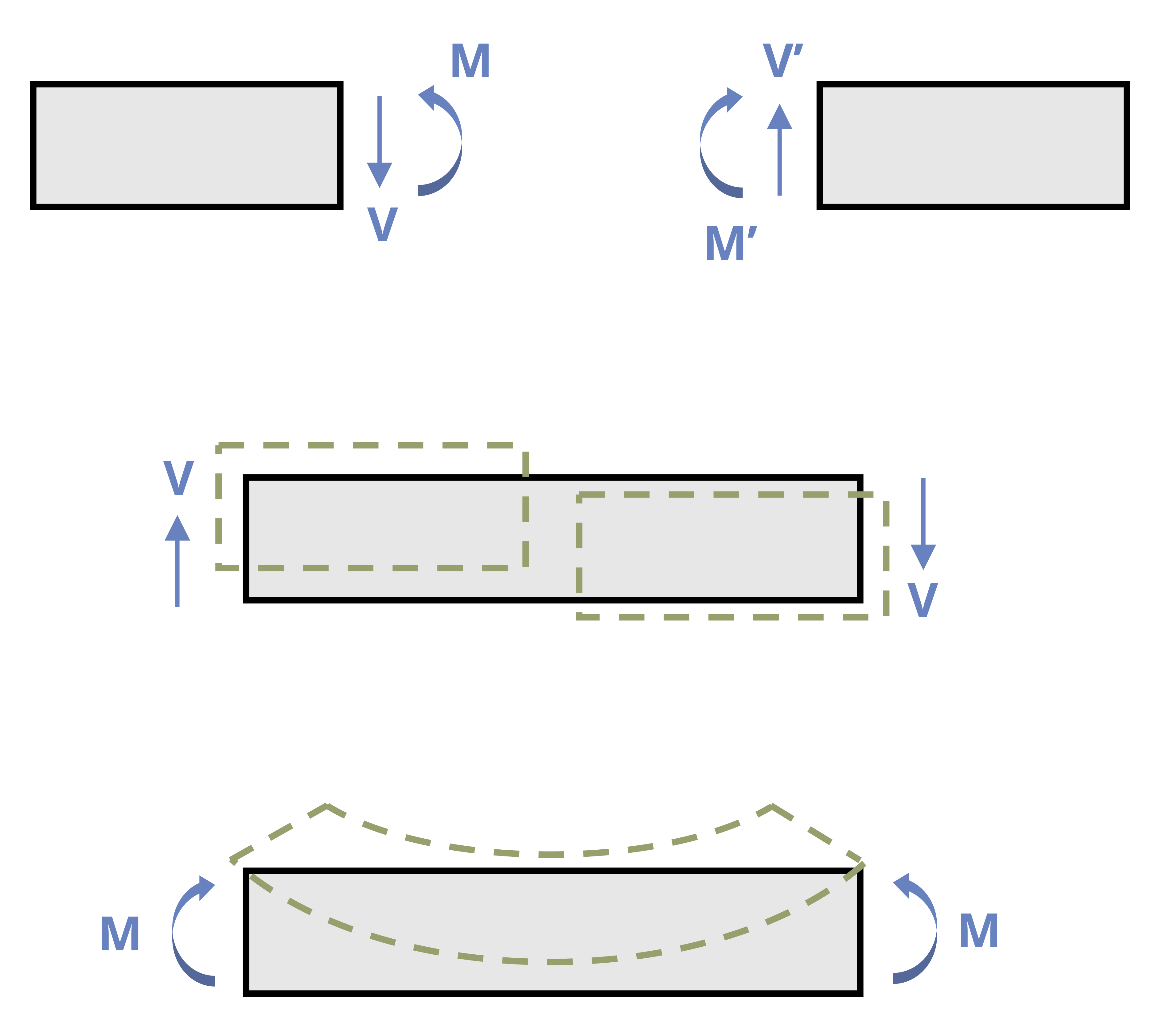
For the purposes of this book, the shear is positive when the external forces shear off as depicted in Figure 7.2. Another way to think about it is that a positive shear is when the internal shear forces cause a clockwise rotation of the beam segment.
The bending moment is positive when the external forces bend the beam in a concave up shape as indicated in Figure 7.2. This causes the top fibers of the beam to be in compression while the bottom fibers are in tension.
7.1 Internal Shear Force and Bending Moment by Equilibrium
Click to expand
One way to find internal shear and bending forces is to cut sections and analyze the free body diagrams (FBDs), as we did in previous chapters of this book. The first step for a statically determinate beam—one where all forces can be found using only equilibrium equations—is to find the external reactions. To determine the internal forces at any point along the beam, we cut the section at that point and draw the FBD from that point to one end of the beam. We’ll include the internal shear force, V, and internal bending moment, M, at the cut section and then use equilibrium equations to solve for those internal loads. This process is demonstrated in Example 7.1.
Example 7.1
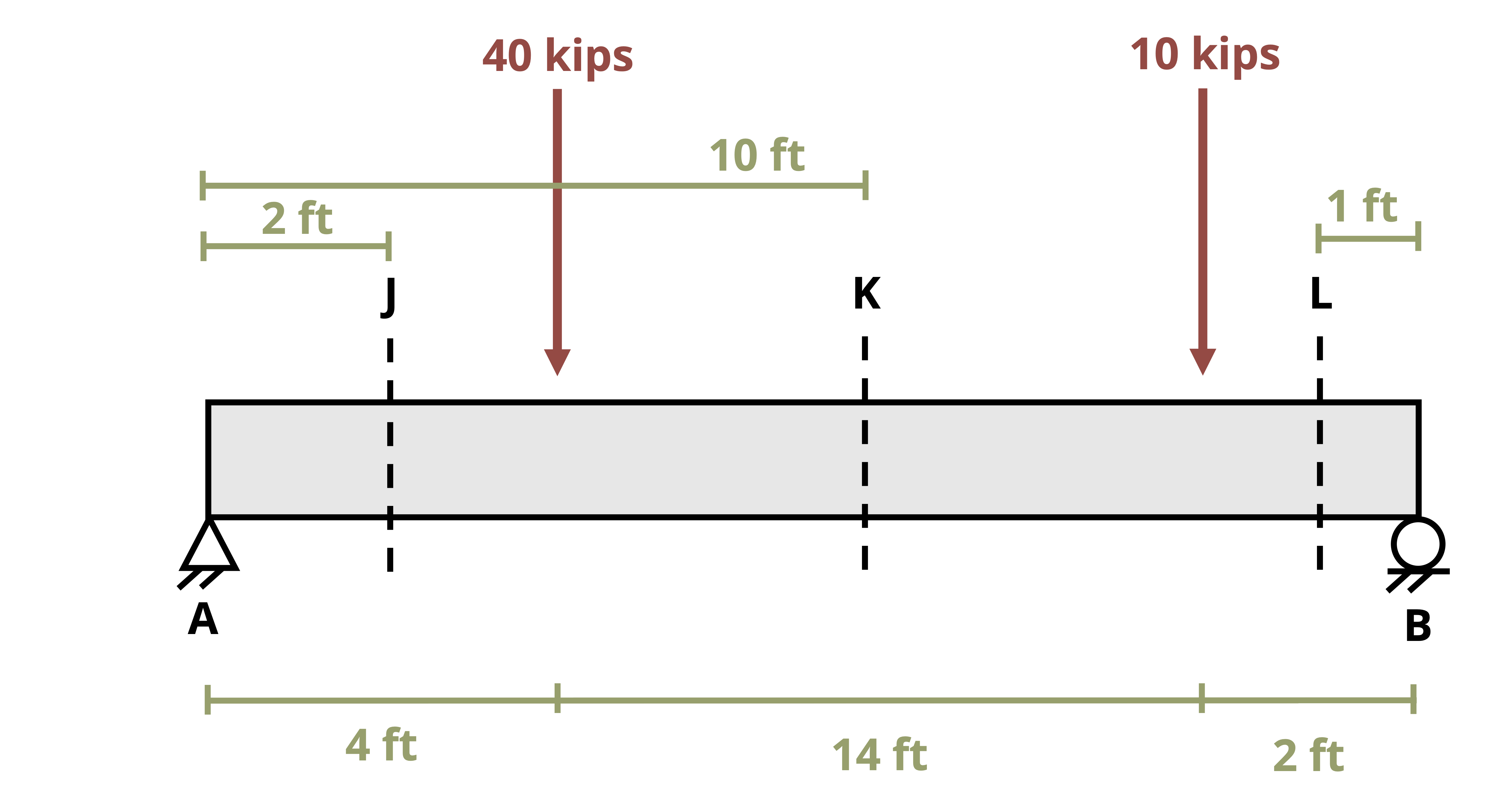
Find the internal shear and bending moment at points J, K, and L in the pictured beam.
The first step is to find the external reactions at the supports A and B.
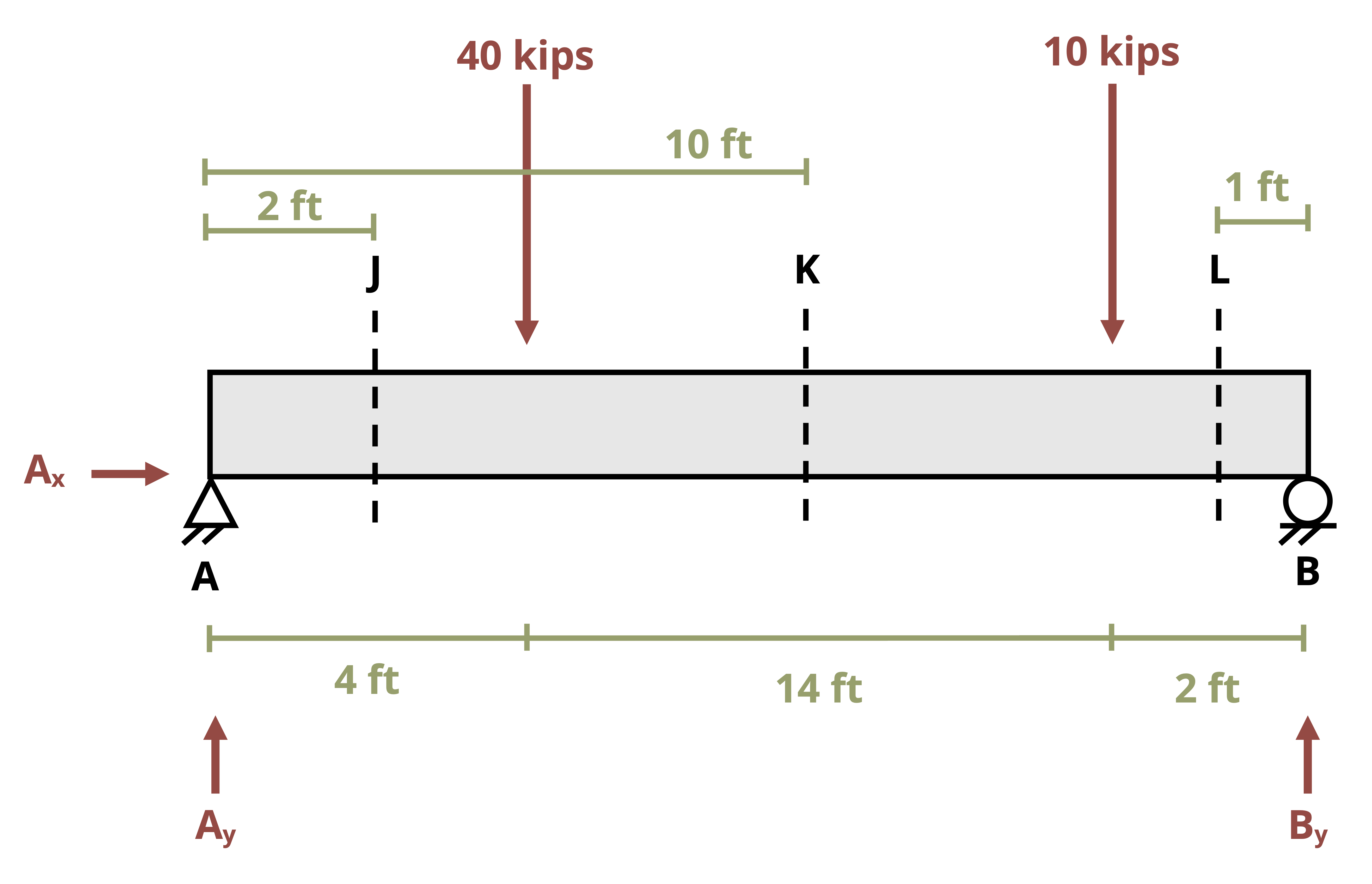
\[ \begin{aligned} & \sum F_x=A_x=0 \\ & \sum M_A=-40{~kips}*4{~ft}-10{~kips}*18{~ft}+B_y*20{~ft}=0 \quad\rightarrow\quad B_y=17{~kips} \\ & \sum F_y=A_y-40-10+17=0 \quad\rightarrow\quad A_y=33{~kips} \end{aligned} \]
Next we draw an FBD of the right end of the beam from point A to J by cutting the beam at section J. The internal forces VJ and MJ are placed at the point of the cut using the positive sign convention. Note that you can assume the direction of these forces since the statics will work out the correct direction.
Section J
To find the internal shear, sum forces in the y direction. To find the internal moment, sum moments at point J.

\[ \begin{aligned} &\sum F_y=33{~kips}-V_J=0 \quad\rightarrow\quad V_J=33{~kips} \\ &\sum M_J=-33{~kips}*2{~ft}+M_J=0 \quad\rightarrow\quad M_J=66{~kip}\cdot{ft} \end{aligned} \]
Section K
To find the internal shear, sum forces in the y-direction. To find the internal moment, sum moments at point K.
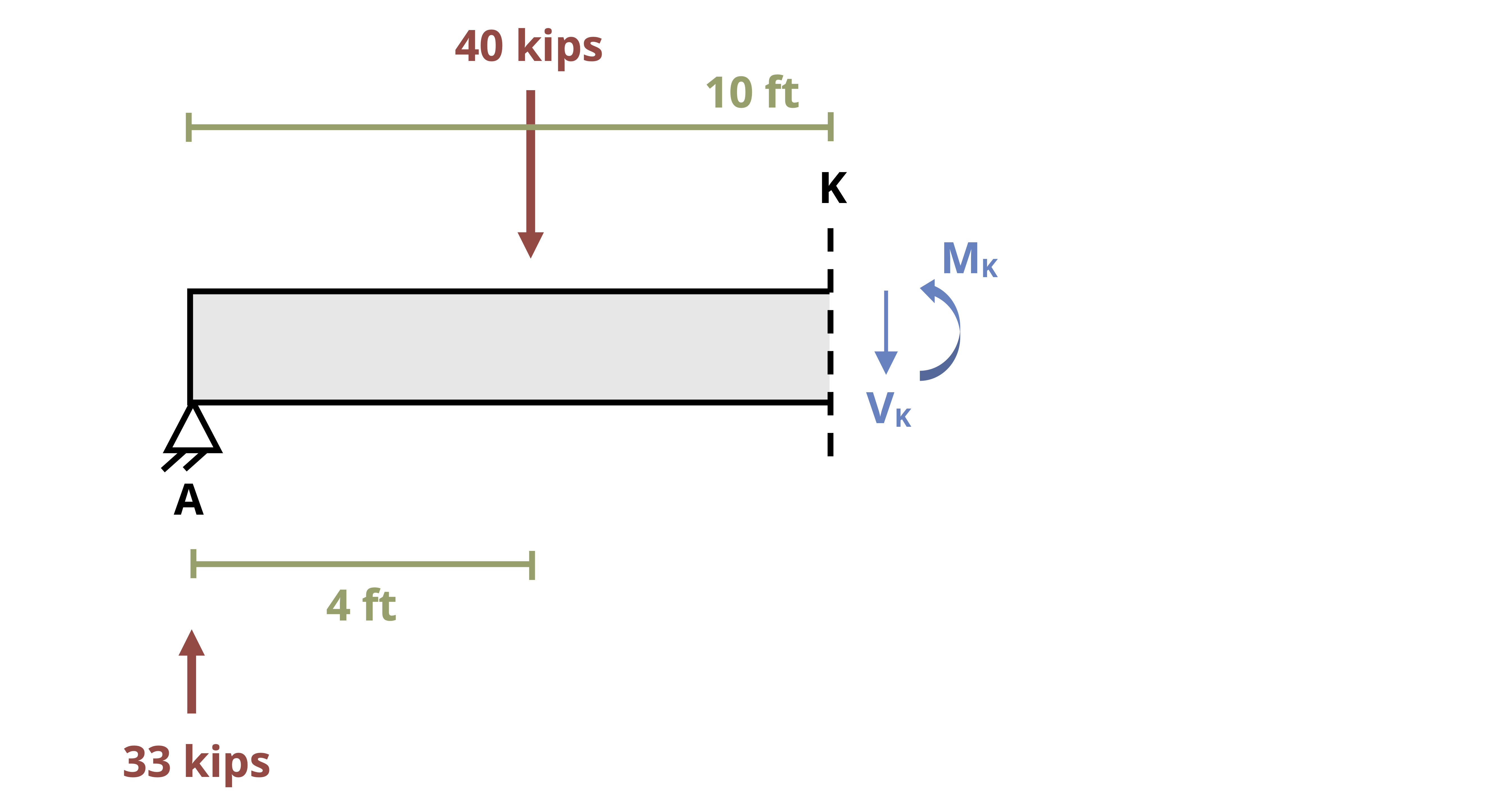
\[ \begin{aligned} &\sum F_y=33{~kips}-40{~kips}-V_k=0 \quad\rightarrow\quad V_k=-7{~kips} \\ &\sum M_k=-(33{~kips}*10{~ft})+(40{~kips}*6{ft})+M_k \quad\rightarrow\quad M_k=90{~kip}\cdot{ft} \end{aligned} \]
Section L
To find the internal shear, sum forces in the y-direction. To find the internal moment, sum moments at point L.
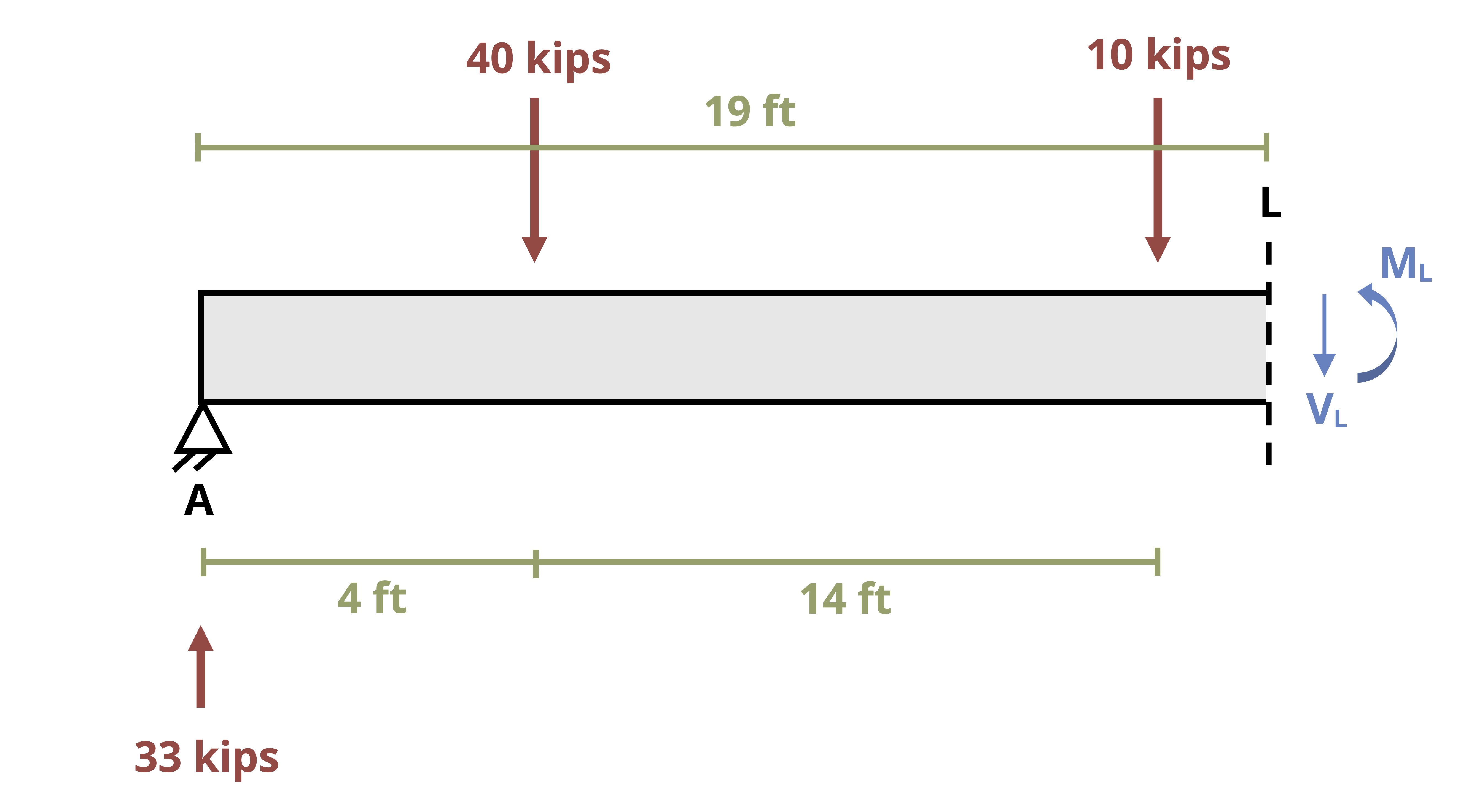
\[ \begin{aligned} &\sum F_y=33{~kips}-40{~kips}-10{~kips}-V_L=0 \quad\rightarrow\quad V_L=-17{~kips} \\ &\sum M_L=-(33{~kips}*19{~ft})+(40{~kips}*15{~ft})+(10{~kips}*1{ft})+M_L=0 \quad\rightarrow\quad M_L=17{~kip}\cdot{ft} \end{aligned} \]
Observe that the internal forces vary at different points along the length of the beam. This method of finding the internal stresses is convenient when the loading is simple or when you know a specific point along the length of the beam. However, as the loading becomes more complex, consider one of the methods outlined in the following sections.
7.2 Relationship Between Load, Shear, and Moment
Click to expand
There is a relationship between loading, shear, and moment—and as shown later in this text, slope and deflection—in a beam. Consider the beam in Figure 7.3, which is subjected to a distributed load, w per unit length.
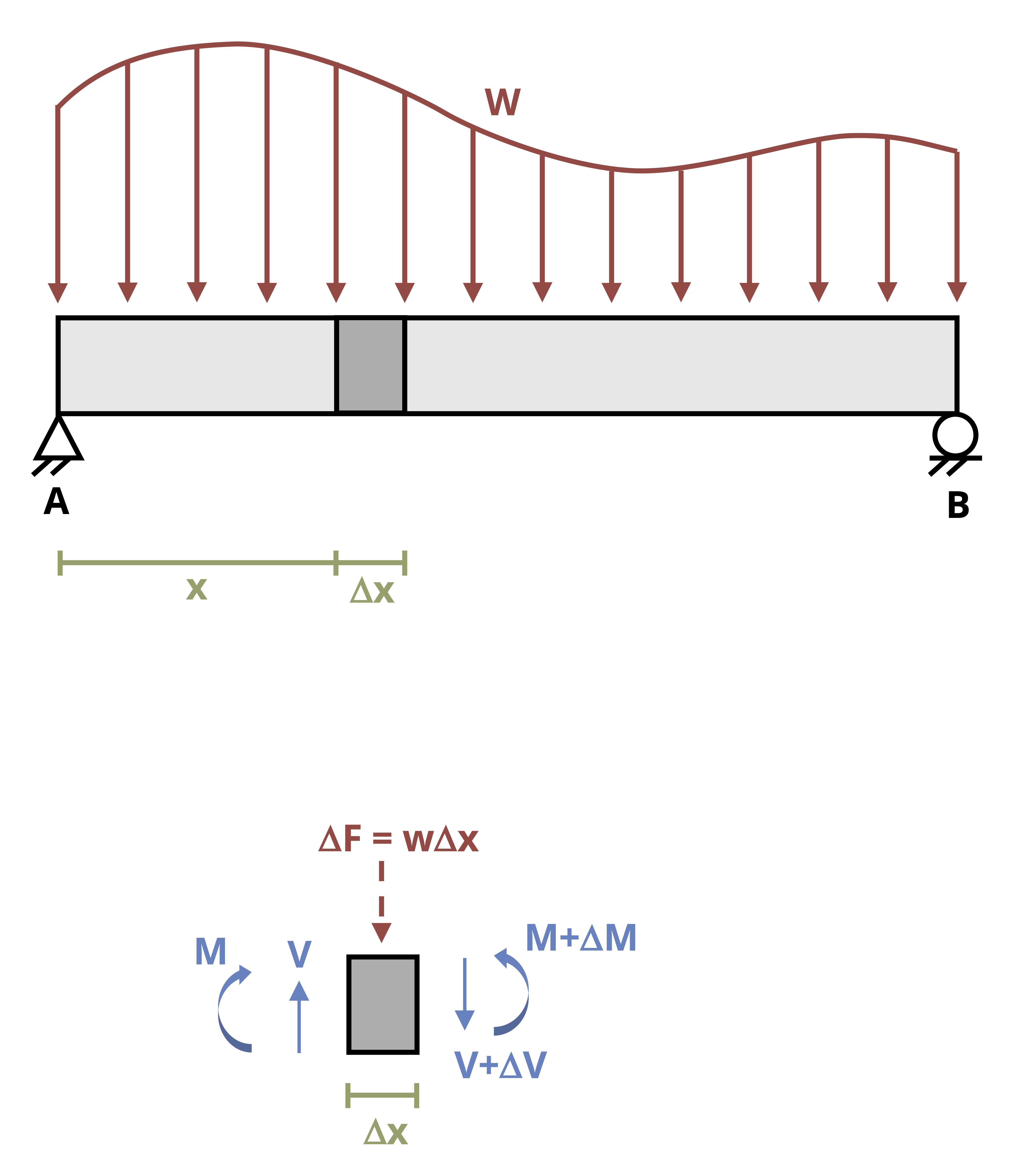
Now look at a small section from that beam that has a width of Δx, shown below. The distributed load has been repalced with a resultant force ΔF (this is indicated by a dashed arrow in the FBD).
Since both sides of the beam have been cut, replace each cut with internal shear and moment forces assuming the positive sign convention established earlier in this chapter.
7.2.1 Relationship Between Load and Shear
This FBD is in static equilibrium, so we can use the equilibrium equation to sum forces in the y direction and set it equal to zero.
\[ \sum F_y=V-\Delta F-(V+\Delta V)=0 \\ \]
\[ \boxed{\Delta V=\Delta F} \tag{7.1}\]
Or \[ \Delta V=w\Delta x \]
Dividing both sides by Δx and then letting Δx approach zero produces
\[ \frac{\Delta V}{\Delta x}=\frac{d V}{d x}=w \]
We then rearrange this by multiplying both sides of the equation by dx.
\[ d V=w d x \]
Now we can integrate between any two points A and B on the beam.
\[ \boxed{\underbrace{\Delta V}_{\substack{\text{change in} \\ \text{shear}}}=\int\underbrace{w d x}_{\substack{\text{area under} \\ \text {loading curve}}}} \tag{7.2}\]
This equation is valid for distributed loads, but not when there is a discontinuity in the shear diagram that is caused by concentrated loads. This relationship should be used only between concentrated loads.
7.2.2 Relationship Between Shear and Moment
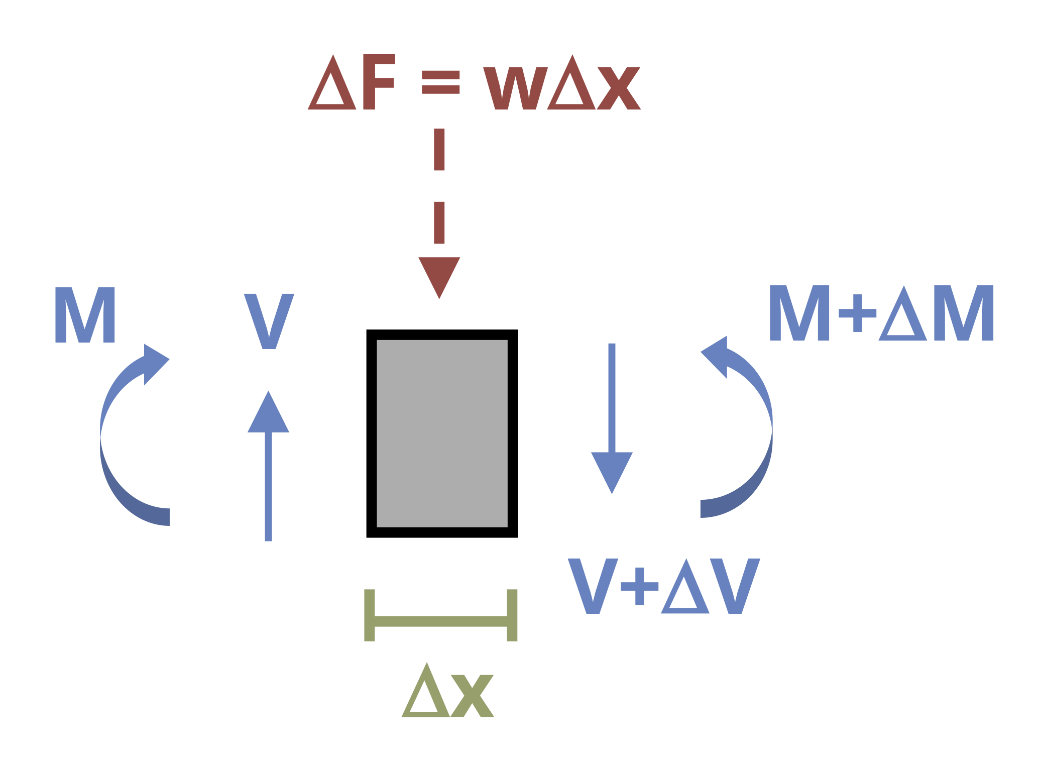
Let’s return to the FBD of the small section of the beam subjected to a distributed load. This segment is shown in Figure 7.4. We can apply another static equilibrium equation, summing moments about point C.
\[ \begin{aligned} \sum M_c=0 & =-M-V(\Delta x)+\Delta F\left(\frac{1}{2} \Delta x\right)+(M+\Delta M) \\ \Delta M & =M+V \Delta x-(w \Delta x)\left(\frac{1}{2} \Delta x\right)-M \\ \Delta M & =V \Delta x-\frac{1}{2} w \Delta x^2 \end{aligned} \]
Dividing both sides by Δx and then letting Δx approach zero yields
\[ \boxed{\underbrace{\frac{\Delta M}{\Delta x}}_{\text { Slope of moment diagram}}=\underbrace{V}_{\text {shear }}} \tag{7.3}\]
Then we rearrange this by multiplying both sides of the equation by dx.
\[ d M=V d x \]
Now it is possible to integrate between any two points A and B on the beam.
\[ \boxed{\underbrace{\Delta M}_{\text {Change in moment}}=\underbrace{\int V d x}_{\text {Area under shear diagram }}} \tag{7.4}\]
This equation is invalid at points where a concentrated force or concentrated moment occurs. These concentrated loads cause discontinuities in the moment diagram.
7.2.3 Using Calculus Knowledge to Build Shear and Moment Diagrams
In a basic sense, the relationship between load, shear, and moment can be described as in Figure 7.5.
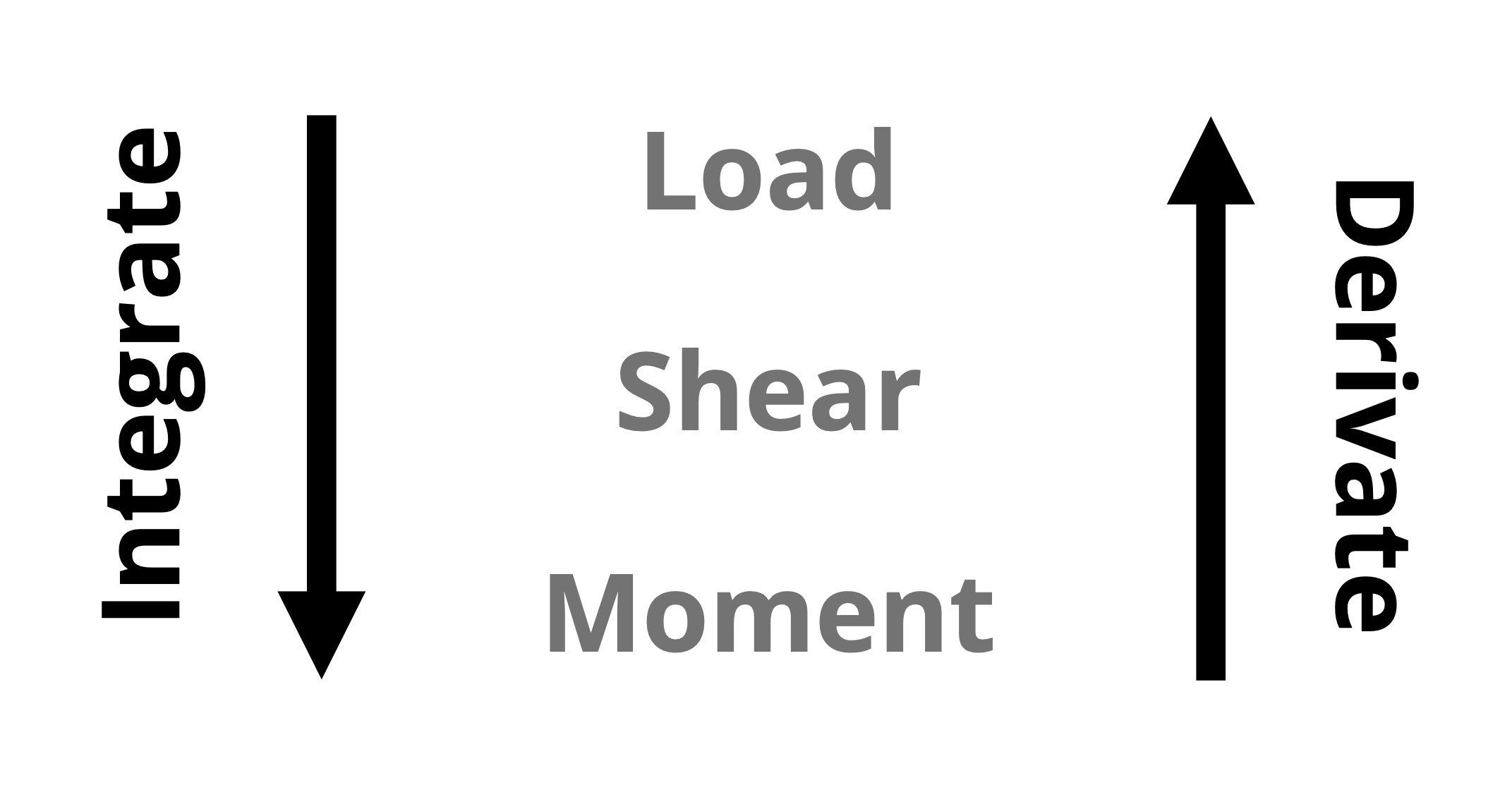
Combine these relationships with what you know about derivatives and integrals from your calculus course. Here are some items of note:
The slope of the shear diagram is equal to the sign and magnitude of the distributed load. If there is no load on a section of the beam, then the slope of the shear diagram is zero.
Similarly, the slope of the moment diagram at any point is the derivative of the moment function evaluated at that point. This is equal to the sign and magnitude of the shear at that point.
The area under the distributed load between two points is equal to the change in the shear between those same two points.
The area under the shear diagram between two points is equal to the change in the moment between those same two points.
The maximum moment occurs where its derivative (shear) is equal to zero.
At the points of concentrated forces, the shear diagram jumps up or down depending on the direction of the force. If the force is up, then the shear diagram will jump up, and if the force is down, the shear diagram will drop down.
At the points of concentrated moments, the moment diagram jumps up or down depending on the direction of the rotation. If the concentrated moment is clockwise, the moment diagram will jump up, and if counterclockwise, it will drop down. This “opposite” direction effect for the internal bending moment is the reaction to the applied moment to stay consistent with the established sign convention. The shear diagram remains unaffected.
If the load can be represented with a polynomial, then we can easily predict the degree of the subsequent shear and moment functions. For example, if the load is a uniformly distributed load (constant), the shear will be a linear function (n + 1) and the moment will be a parabola (n + 2).
Use all you know about calculus and the relationships between functions when you derive and integrate to build, check, and analyze shear and moment diagrams.
7.3 Determining Equations by Equilibrium
Click to expand
The relationship between load, shear, and moment allows us to build complete shear and moment diagrams using a few different methods. We’ll explore two of them: an equilibrium method and a graphical method.
In Section 7.1 we found the internal shear force and bending moment at specific points in the beam by cutting a cross-section at a given point and using equilibrium. The method in this section is similar, but instead of cutting a cross-section at a specific point, we’ll cut a cross-section at distance x from the left end of the beam. We’ll draw an FBD and determine the internal shear force (V) and bending moment (M) as before, but this time the resulting equations for V and M will be functions of distance x.
To draw the diagrams, we can solve this equation at two values of x. It is often simplest to solve when x = 0 and when x = L, the length of the beam. These are two points we can then connect on our diagram. The diagram’s shape depends on the highest power of x that appears in the equation.
For x0 we obtain a flat horizontal line.
For x1 we obtain a straight diagonal line.
For x2 we obtain a curved line.
For x3 we obtain a cubic curve.
If two points are insufficient to determine the exact shape of the curve, simply solve the equations at a third point (e.g., where x = L/2). We can solve the equations at as many points as necessary, but two or three points, along with knowledge of the general shape of the line, are typically sufficient. The equations found using this method are valid as long as the external loading doesn’t change.
Cases where the external loading does change require us to determine a new set of equations each time the loading changes. This includes any time a distributed load begins or ends, and both sides of a concentrated force or couple. In each region of load, we will cut a cross-section at distance x and determine equations for V and M that are valid for that region. We can then solve each equation at values of x at the start and end of their valid region and build up the complete shear force and bending moment diagrams.
Example 7.2 illustrates this method for a simply supported beam, and Example 7.3 for a cantilever beam.
Example 7.2
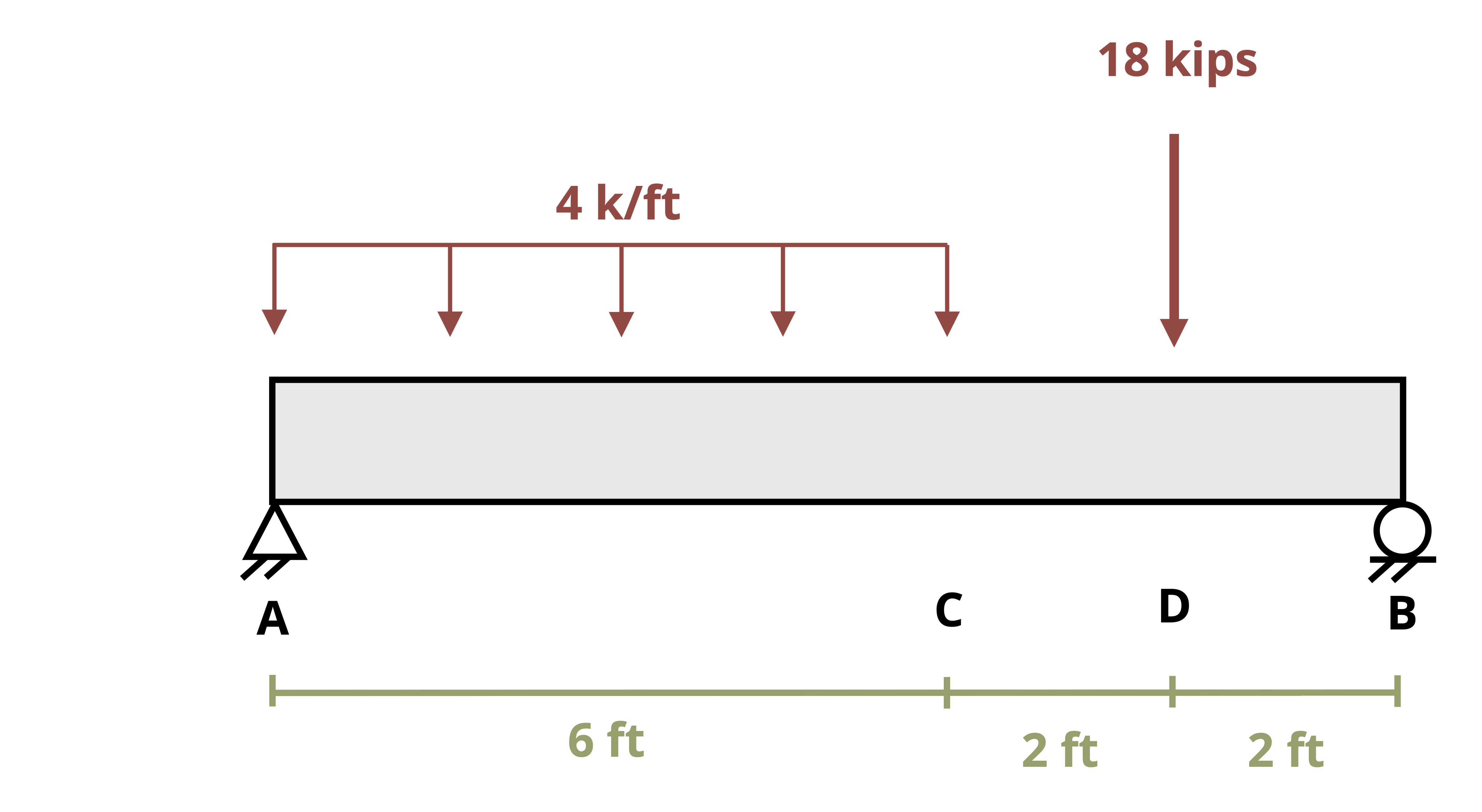
Draw the shear force and bending moment diagrams for the beam shown.
The first step is to draw an FBD of the beam, being sure to change the supports to the correct external reaction forces as shown.
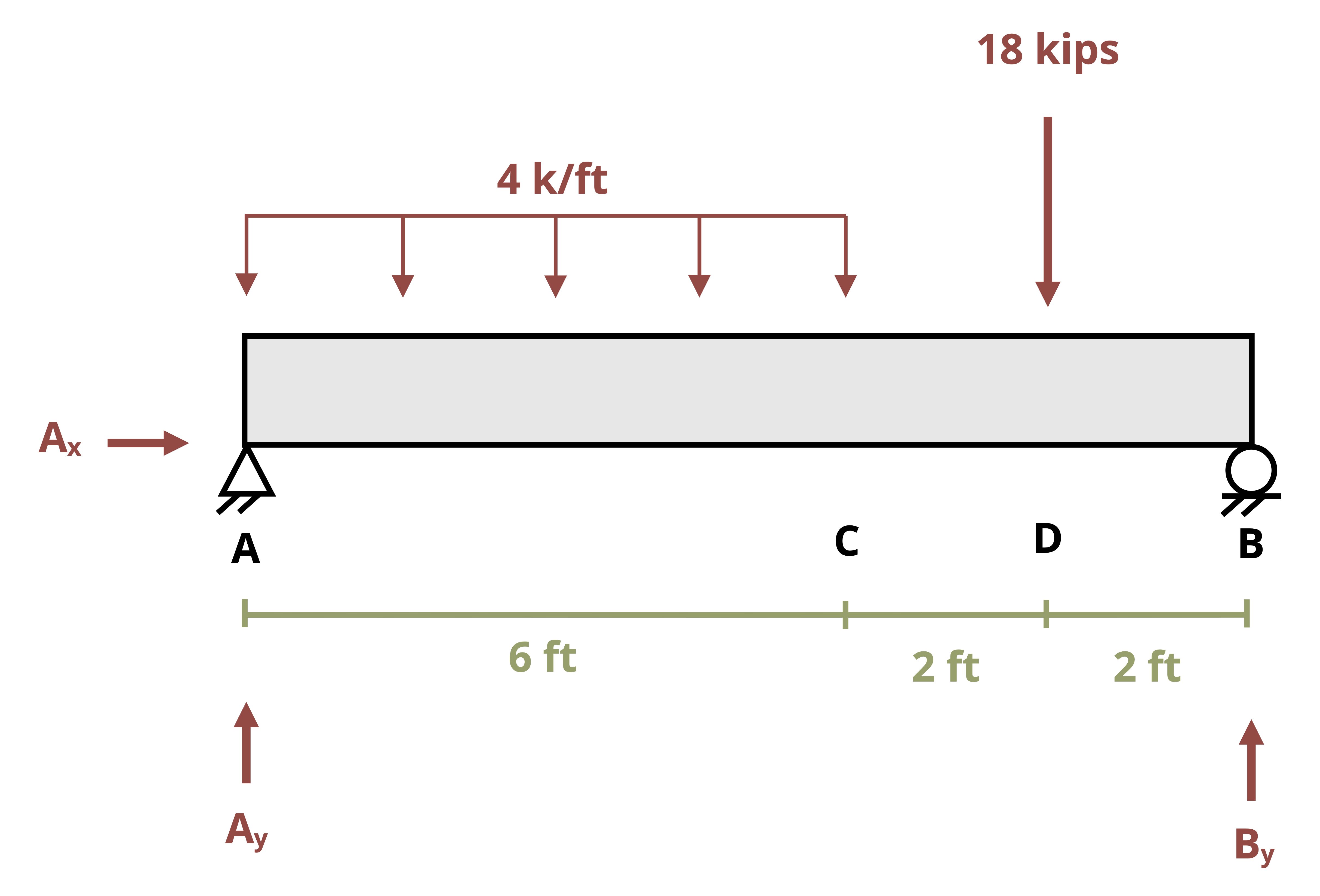
We then use static equilibrium equations to solve for the magnitude of the support reactions.
\[ \begin{aligned} &\sum F_x=A_x=0 \\ &\sum M_A=-4\frac{kips}{ft}*6{~ft}*3{~ft}-18{~kips}*8{~ft}+B_y*10{~ft}=0 \quad\rightarrow\quad B_y =21.6{~kips} \\ &\sum F_y=A_y-4\frac{kips}{ft}*6{~ft}-18{~kips}+21.6{~kips}=0 \quad\rightarrow\quad A_y =20.4{~kips} \end{aligned} \]
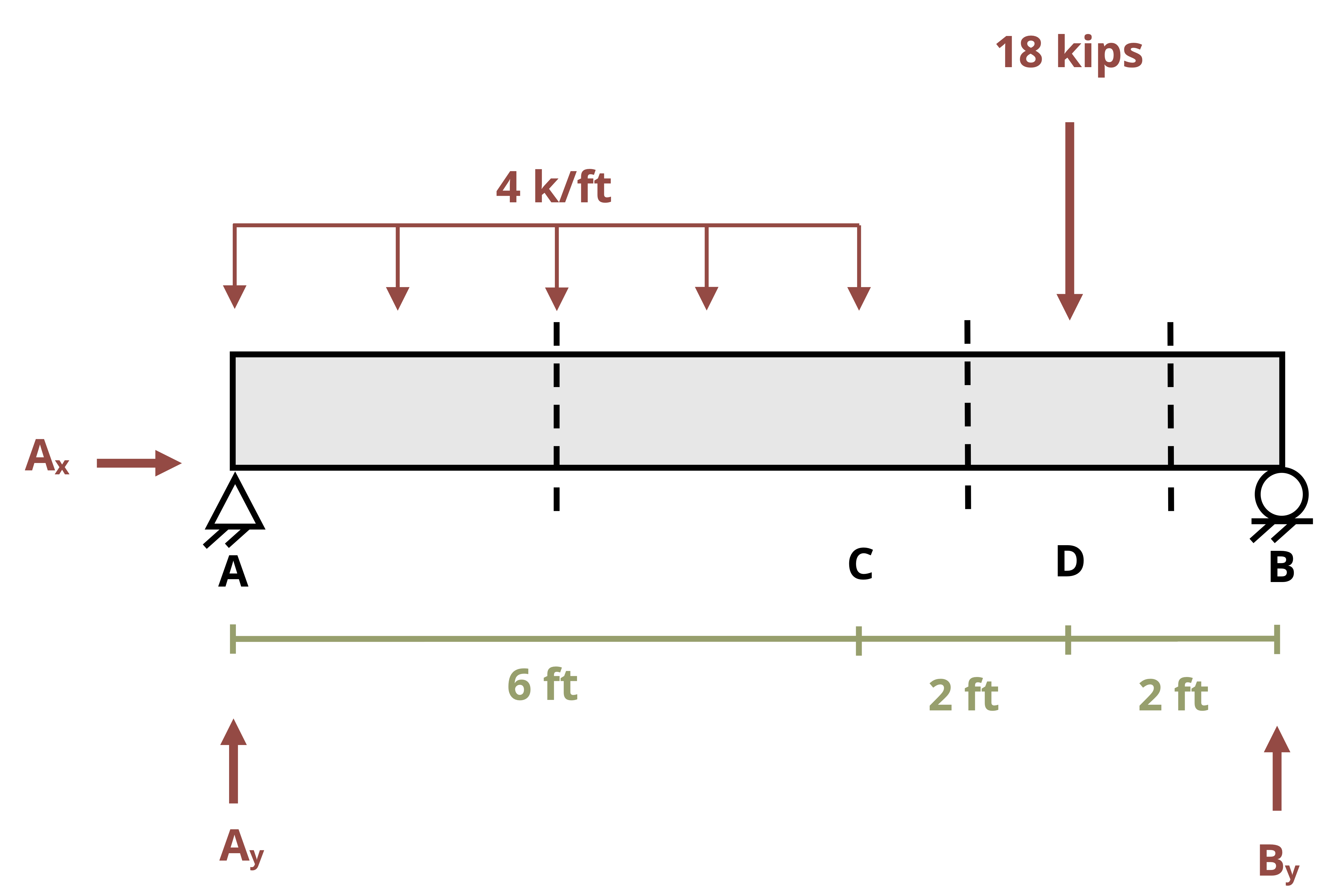
Next we cut a cross-section within the loading region concerned. When choosing sections, be sure to cut within the uniform load and between loads and reactions. For this example, here we must cut three sections to create the complete shear and moment diagram. These sections are depicted with the green lines. Then the equilibrium equations are used to find the internal shear force as a function of x, V(x).
Section between A and C
\[ \begin{aligned} &\sum F_y=20.4-4(x) -V=0 \quad\rightarrow\quad V(x)=-4 x+20.4 \\ &\sum M_0=-20.4(x)+4(x)\left(\frac{x}{2}\right)+M=0 \quad\rightarrow\quad M(x)=-2 x^2+20.4 x \\ \end{aligned} \]
Note that you can easily check the statics because V(x) is the derivative of M(x). For polynomials, this is a quick test to see if the equations make sense.
We plot the V(x) and M(x) equations on an axis from x = 0 to x = 6 ft. Solving the equations at these points yields
\[ \begin{aligned} &V(0)=-4(0)+20.4=20.4{~kips} \\ &V(6)=-4(6)+20.4=-3.6{~kips} \\ &M(0)=-2(0)^2+20.4(0)=0 \\ &M(6)=-2(6)^2+20.4(6)=50.4{~kip}\cdot{ft} \end{aligned} \]
Note that the shear diagram is drawn directly below the beam, and the moment diagram directly below the shear. These three—load, shear, and moment—share the same x-axis, whereas the vertical axes for the shear (V) and moment (M) diagrams have different units and possibly different scales.
Drawing the shear and moment diagrams directly below the beam is good practice so that you can get a complete picture of what is going on along the length of the beam.
Section between C and D
\[ \begin{aligned} \sum &F_y=20.4-4(6)-V=0 \quad\rightarrow\quad V(x)=-3.6 \\ \sum &M_0=-20.4(x)+4(6)(x-3)+M=0 \\ &M(x)=+20.4 x-24 x+72 \\ &M(x)=-3.6 x+72 \\ \end{aligned} \]
We then add the section from C to D using the V(x) and M(x) equations. Notice that since there are no applied loads on the beam from C to D, the shear diagram remains constant. This means the moment diagram is linear between x = 6 and x = 8 ft.
\[ \begin{aligned} &V(6)=-3.6{~kips} \\ &M(6)=-3.6(6)+72=50.4{~kip}\cdot{ft} \\ &V(8)=-3.6 {kips} \\ &M(8)=-3.6(8)+72=43.2{~kip}\cdot{ft} \\ \end{aligned} \]
Section between D and B

\[ \begin{aligned} \sum &F_y = 20.4-4(6)-18-V=0 \quad\rightarrow\quad V(x) =-21.6 \\ \sum &M_0 =-20.4(x)+4(6)(x-3)+18(x-8)+M=0 \\ & M(x) =20.4 x-24 x+72-18 x+144 \\ &M(x) =-21.6 x+216 \end{aligned} \]
Finally, we graph the V(x) and M(x) equations obtained from point D to point B (x = 8 to x = 10 ft).
\[ \begin{aligned} &V(8)=-21.6{~kips} \\ &M(8)=-21.6(8)+216=43.2{~kip}\cdot{ft} \\ &V(10)=-21.6{~kips} \\ &M(10)=-21.6(10)+216=0 \\ \end{aligned} \]
You now have complete shear and moment diagrams. Be sure to label the axes, including units, and all pertinent values.
These diagrams are used in the design of the beam and its components.
Note that in this example, the entire length of the beam is subjected to positive moment. According to the sign convention at the beginning of this chapter, remember, a positive moment indicates a concave up behavior. Given the beam and the external loads, this makes sense, for the beam will want to bend concave up between supports, as the figure shows.
Example 7.3
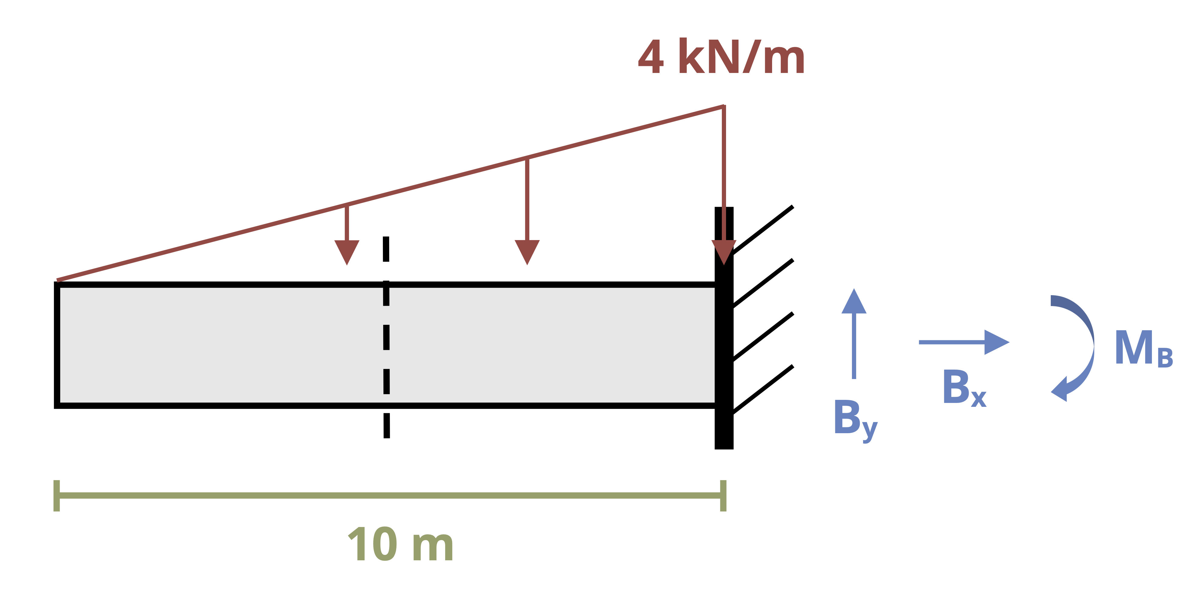
Draw the shear force and bending moment diagrams for the beam shown.
The first step is to draw an FBD of the beam, being sure to change the supports to the correct external reaction forces.
We then use static equilibrium equations to solve for the magnitude of the support reactions.
\[ \begin{aligned} &\Sigma F_x=B_x=0 \\ &\Sigma F_y = -\frac{1}{2}(10~m)\left(4~\frac{kN}{m}\right) + B_y=0 \quad\rightarrow\quad B_y=20~kN \\ &\Sigma M_B=\frac{1}{2}(10~m)\left(4~\frac{kN}{m}\right)\left(\frac{10~m}{3}\right)-M_B=0 \quad\rightarrow\quad M_B=66.7 kN \cdot m \end{aligned} \]
Next we cut a cross-section within the loading region concerned. For this example, we cut one section between A and B to create the complete shear force and bending moment diagram. This section is depicted with the dashed line. Then equilibrium equations are used to find the internal shear force as a function of x, V(x).
Section between A and B
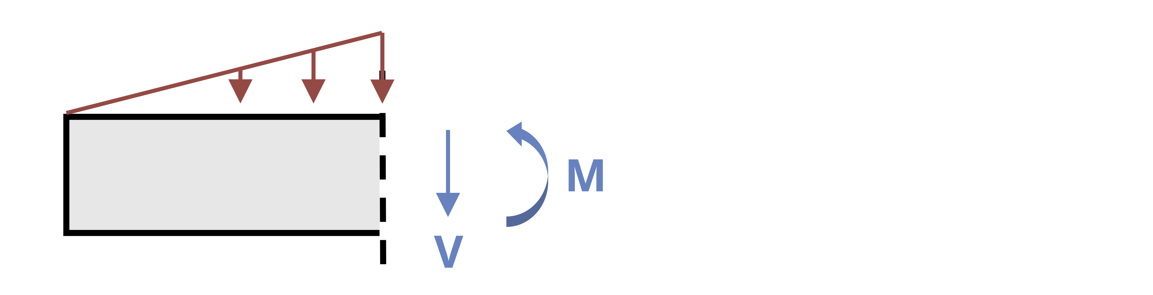
\[ \Sigma F_y=-V-\frac{1}{2}(x)\left(\frac{4}{10}x\right)=0 \\ V(x)=-\frac{1}{5}x^2 \\ \Sigma M=\frac{1}{2}(x)\left(\frac{4}{10}\right)\left(\frac{1}{3}x\right)+M=0\\ M(x) = -\frac{1}{15}x^3 \]
Note that you can easily check the statics because V(x) is the derivative of M(x). For polynomials, this is a quick test to see if the equations make sense.
We plot the V(x) and M(x) equations on an axis from x = 0 to x = 10 m. Notice how the shear diagram is drawn directly below the beam, and the moment diagram directly below the shear. These three—load, shear, and moment—share the same x-axis, whereas the vertical axes for the shear (V) and moment (M) diagrams have different units and possibly different scales.
Drawing the shear and moment diagrams directly below the beam is good practice so that you can get a complete picture of what is going on along the length of the beam.
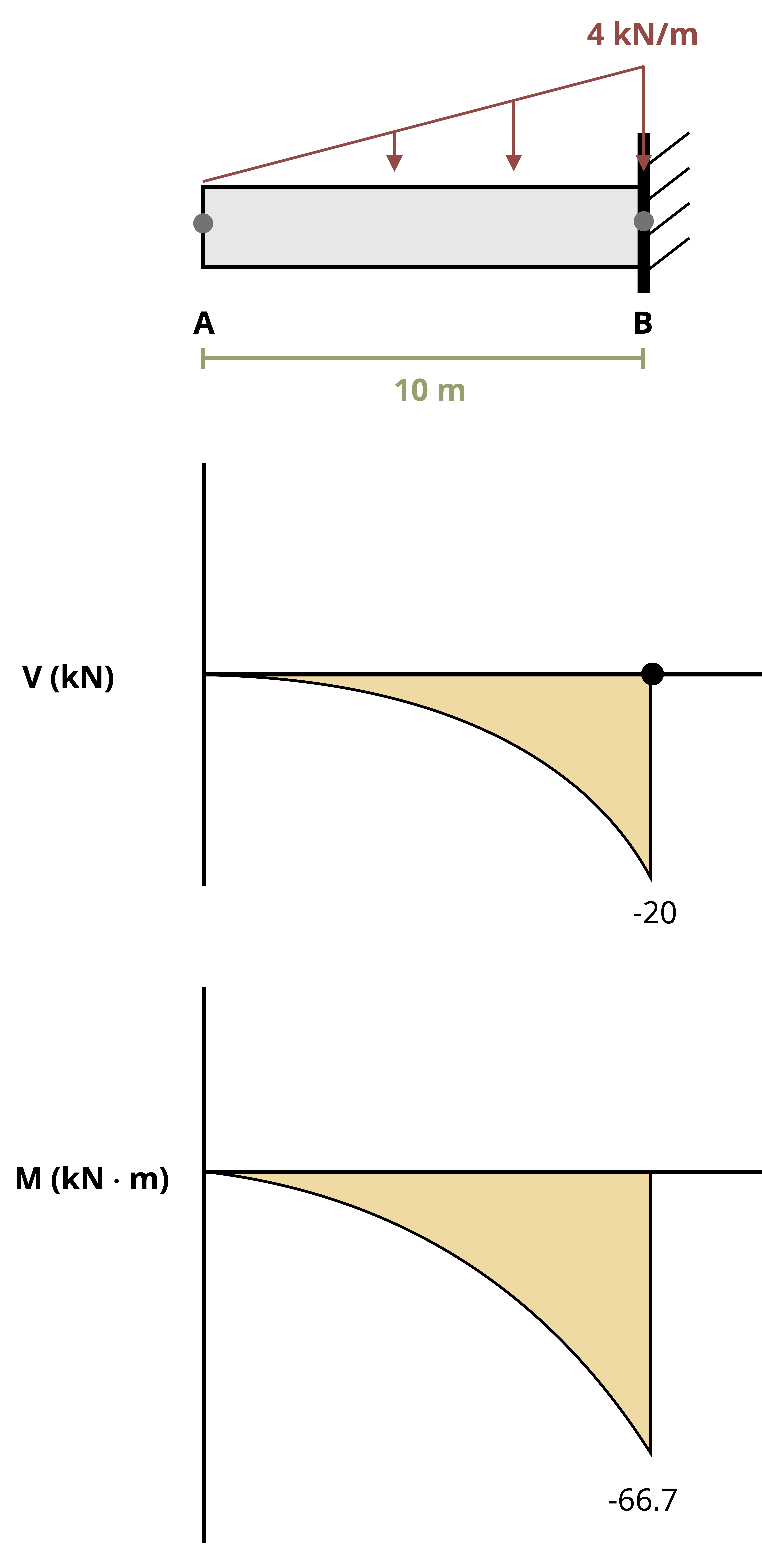
See that the shear diagram starts at zero, then at X = 10 m, V(10) = -20 kN. The reaction calculated was 20 kN going up, so adding that reaction closes the shear diagram.
Similarly, the moment diagram is the graph of the cubic equation from x = 0 to x = 10. M(10) = -66.7 kN·m is the same as the reaction calculated to close the moment diagram.
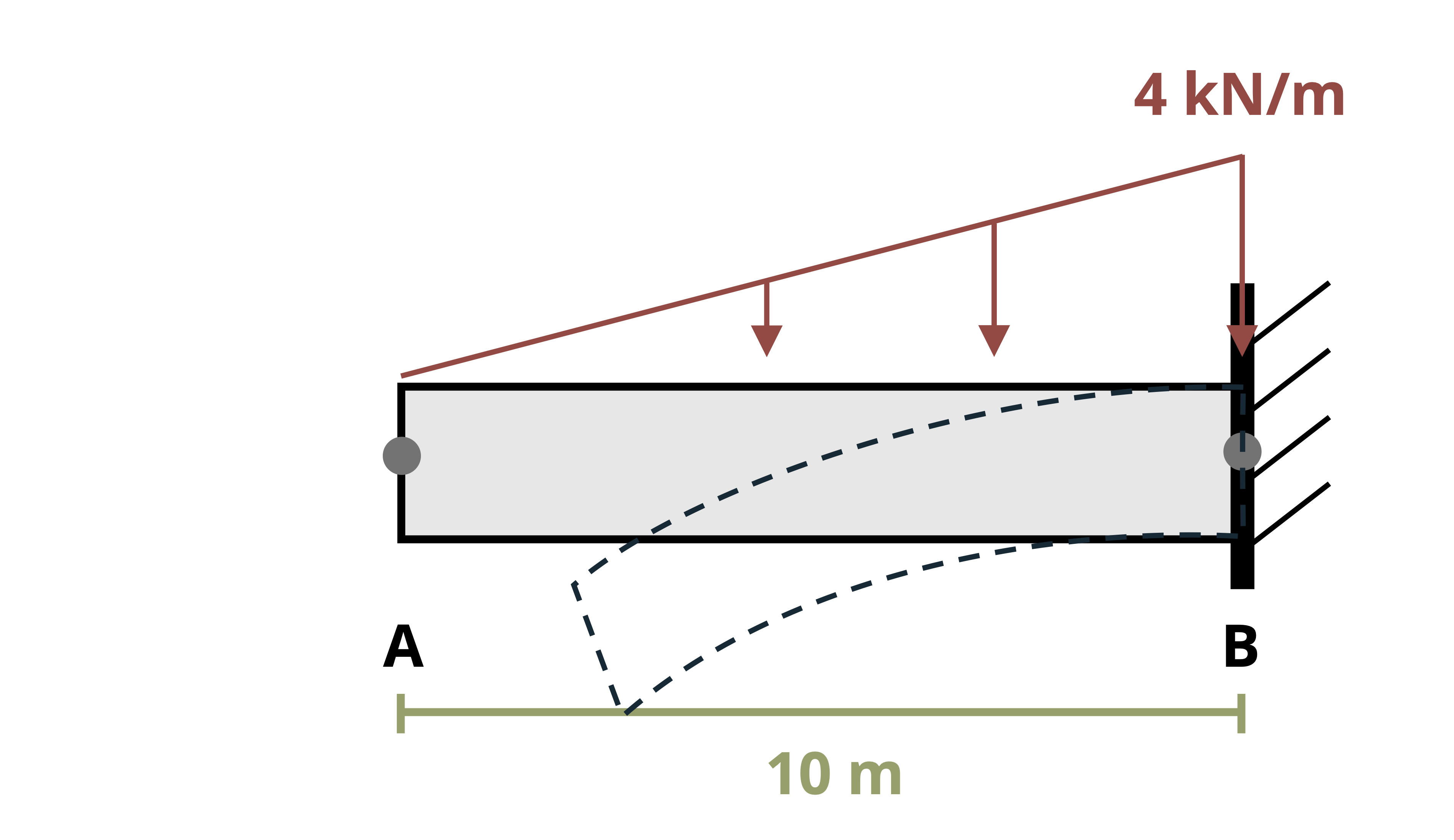
Note that in this example the entire length of the beam is subjected to negative moment. According to the sign convention presented at the beginning of this chapter, remember, a negative moment indicates a concave down behavior. Given the beam and the external loads, this makes sense because the beam will want to bend concave down, as shown in the figure.
7.4 Graphical Method Shear Force and Bending Moment Diagrams
Click to expand
An alternative, often faster method for drawing shear force and bending moment diagrams is the graphical method. This approach leverages the relationships between load, shear force, and bending moment, allowing us to derive one diagram from another.
Specifically, Section 7.2 showed that \(\frac{dV}{dx}=w\) and \(\frac{dM}{dx}=V\). That is, the slope of the shear force diagram at any point equals the applied distributed load at that point, and the slope of the bending moment diagram at any point equals the shear force at that point.
Further, any applied concentrated force causes a jump in the shear diagram (e.g., an upward force results in an upward jump). Any applied couples causes a jump in the bending moment diagram (e.g., a clockwise moment causes an upward jump). Thus the shape of the shear force diagram is based on the applied loads, and the shape of the bending moment diagram is based on the shear force diagram.
Finally, Equation 7.2 also showed that the change in shear force between any two points is equal to the area under the distributed load between those same two points. Evident from Equation 7.4 is that the change in bending moment between any two points is equal to the area underneath the shear force diagram between those two points. This allows us to add numbers to the diagrams and determine the value of the shear force and bending moment at key points.
When the loading is relatively simple, consisting of concentrated forces, concentrated moments, and uniformly distributed loads, we can use geometry to find the area of the load and shear diagrams since the shapes are simple. Example 7.4 and Example 7.5 illustrate this method.
Example 7.4
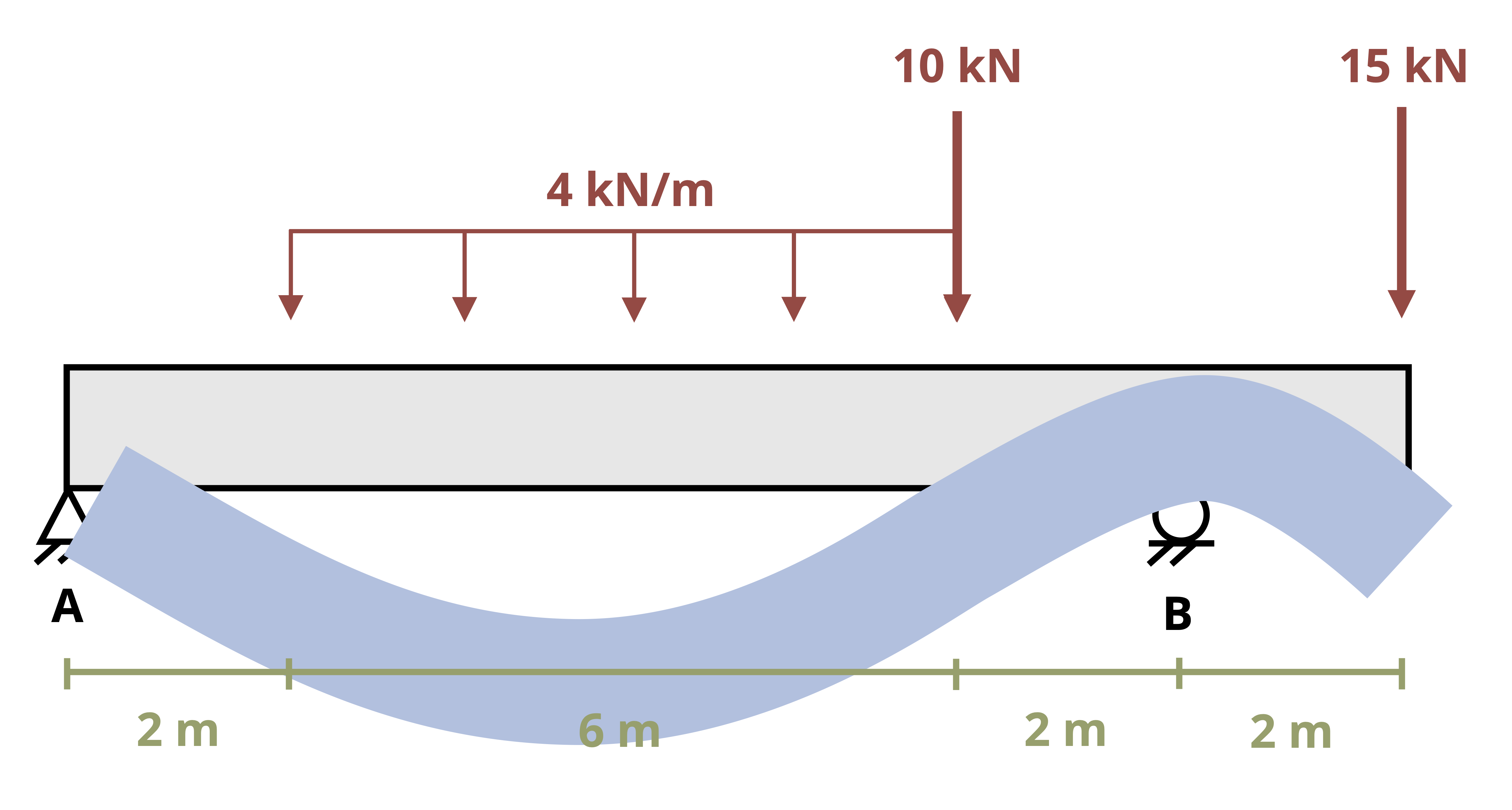
Draw the shear force and bending moment diagrams for the beam shown.
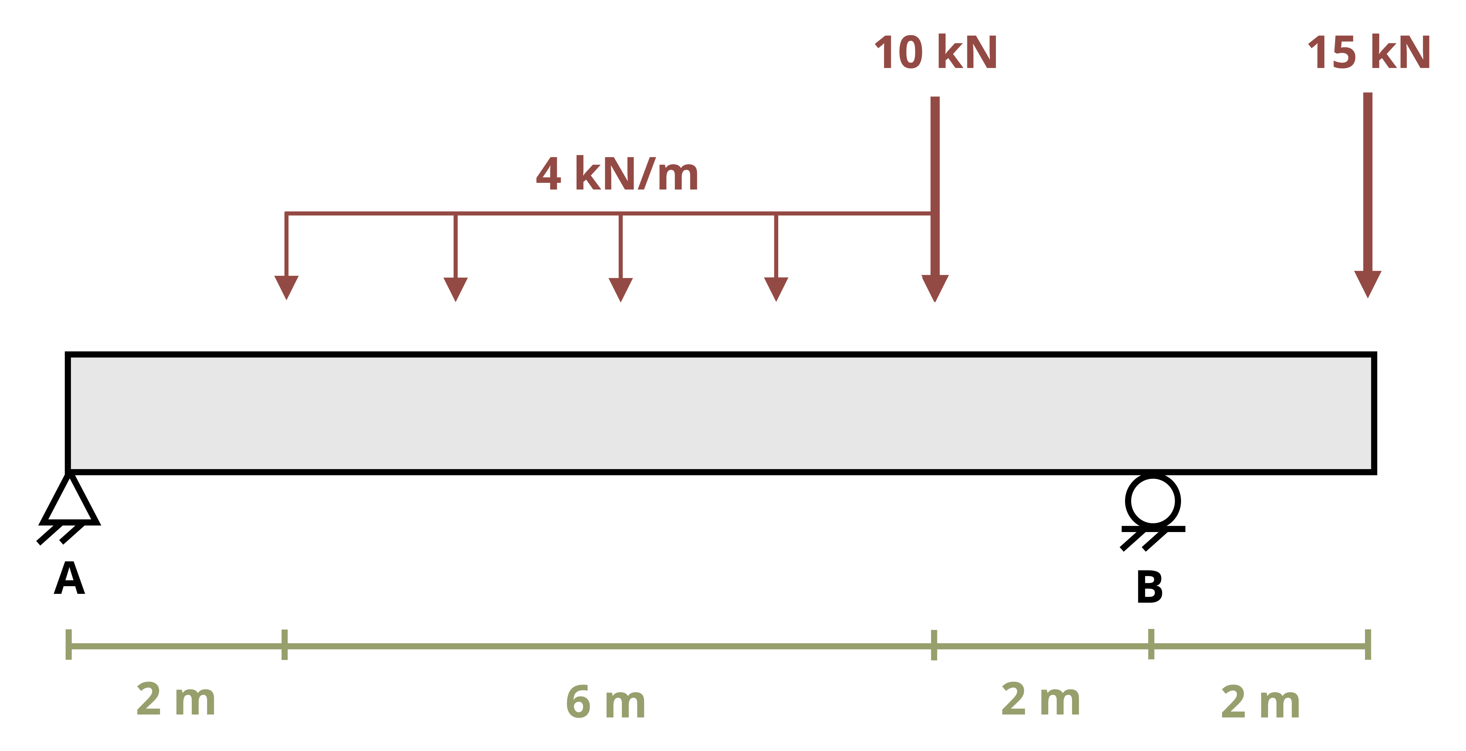
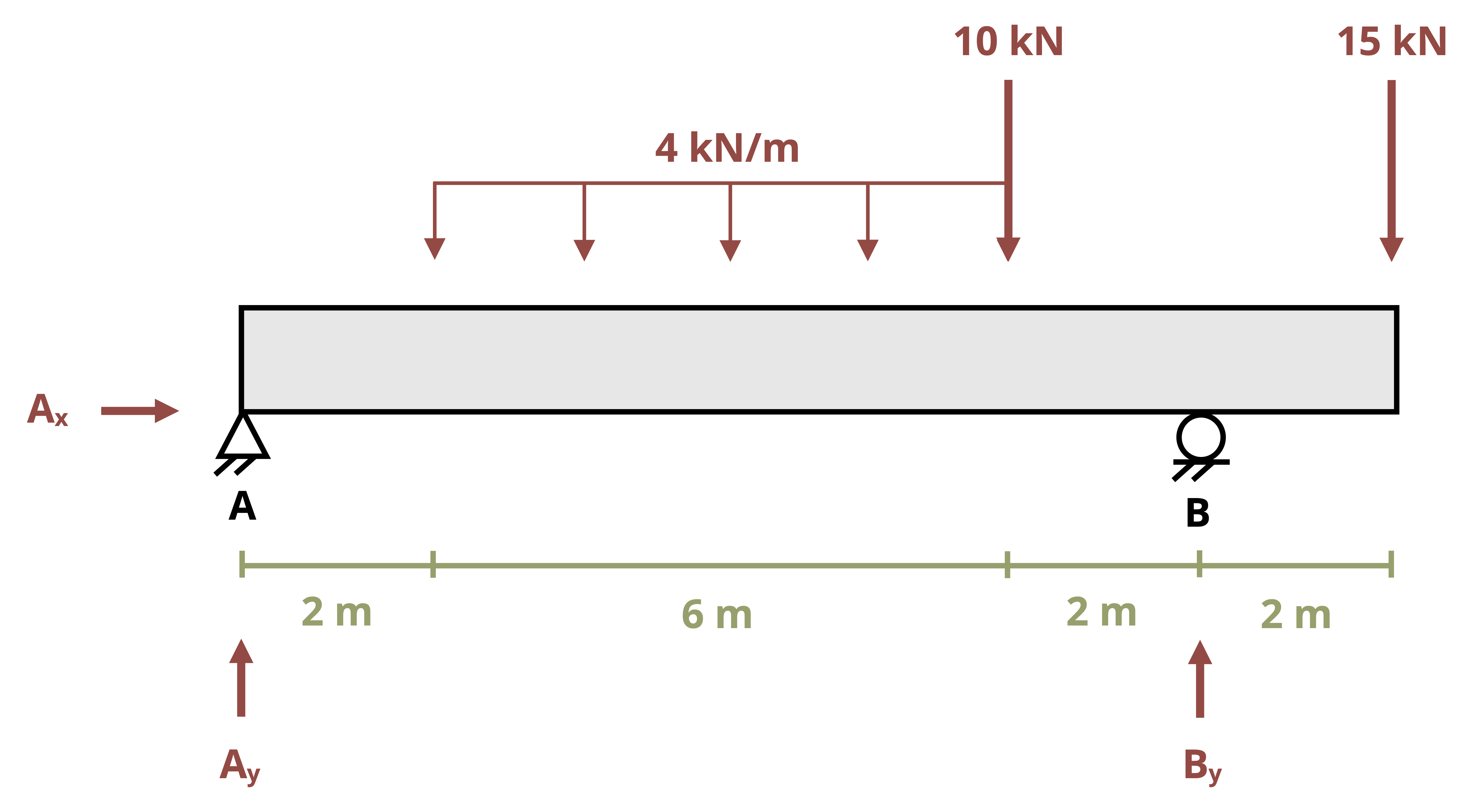
The first step is to draw an FBD of the beam, being sure to change the supports to the correct external reaction forces, as shown below.
Then use static equilibrium equations to solve for the magnitude of the support reactions.
\[ \begin{aligned} &\sum F_x=A_x=0 \\ &\sum M_A=-4\frac{kN}{m}(6{~m})(5{~m})-10{~kN}(8{~m})+B_y(10{~m})-15{~kN}(12{~m})=0 \quad\rightarrow\quad B_y =38{~kN} \\ &\sum F_y=A_y-4\frac{kN}{m}(6{~m})-10{~kN}-15{~kN}+38{~kN} \quad\rightarrow\quad A_y =11{~kN} \end{aligned} \]
Now that the external forces are known, build the shear diagram. Start at the leftmost point of the beam, point A.
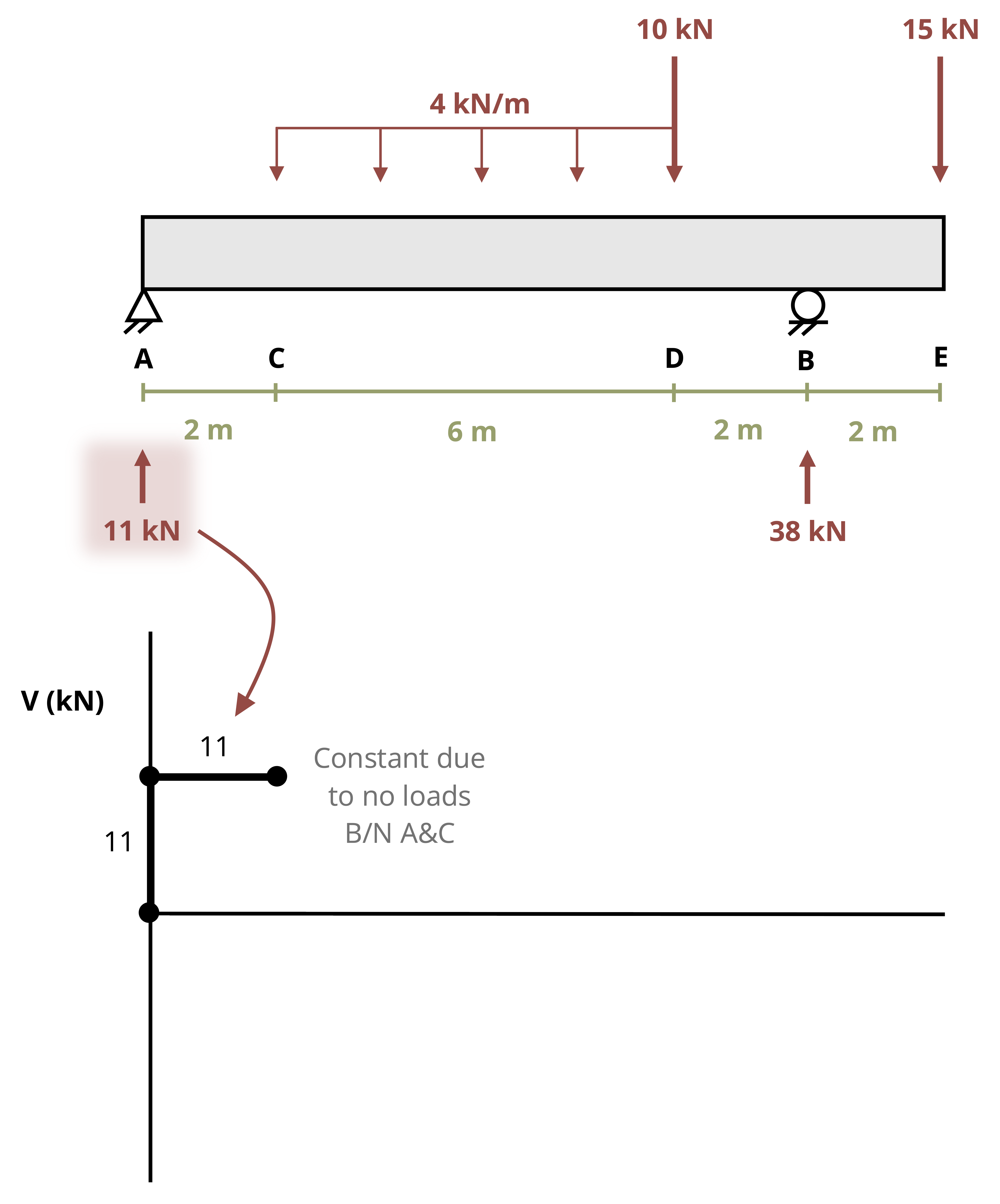
The first force encountered is at point A, the reaction force of 11 kN. The force is going up, so do that same thing on the shear diagram.
From that point, look at the beam and note that no forces are acting between points A and C. This indicates the shear diagram will remain constant at 11 kN.
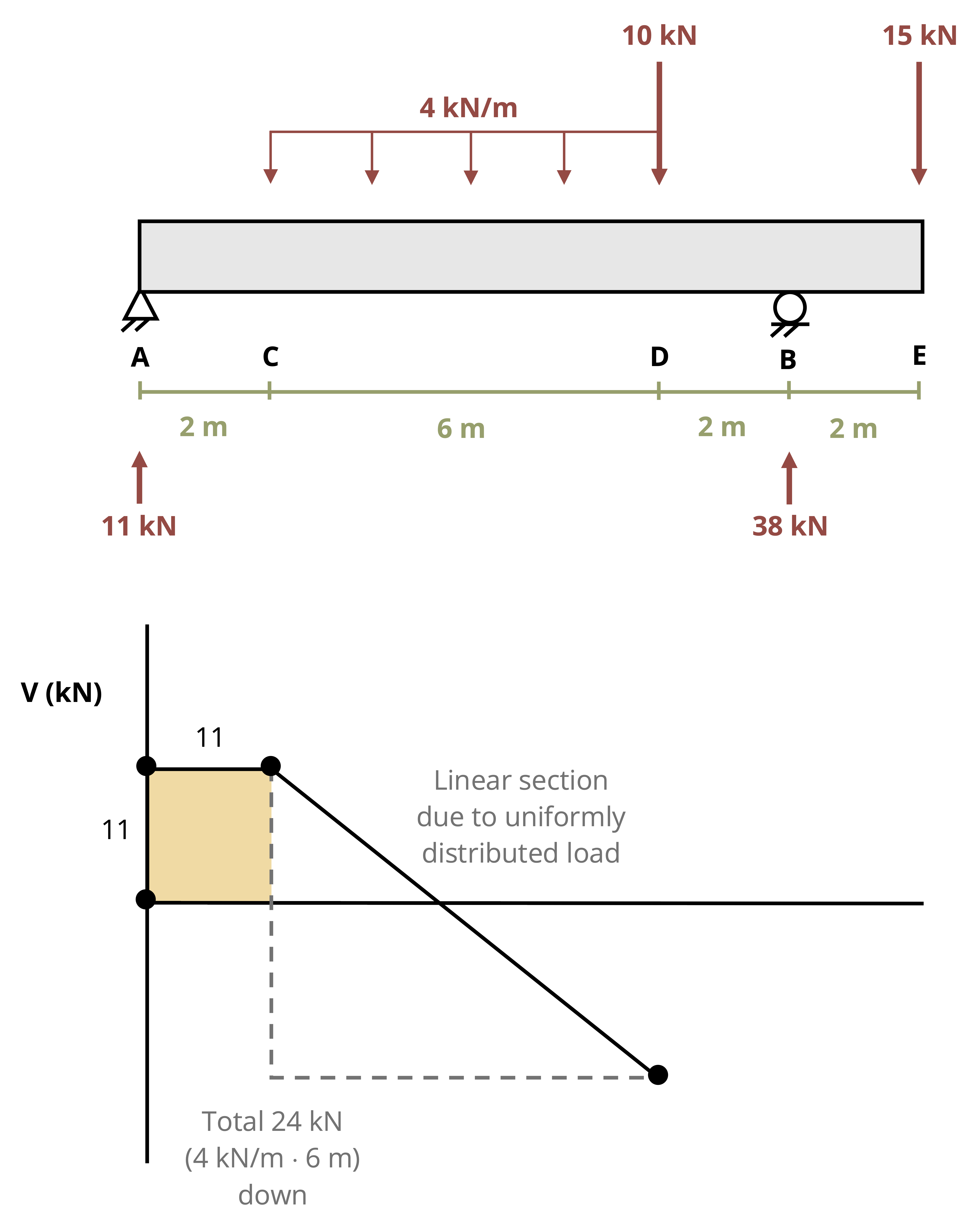
The 4 kN/m uniformly distributed load starts at point C and goes for 6 m until point D. The force is going down for a total of 24 kN (4 kN/m·6 m). Since the load is constant from point C to D, the shear will be linear between those points. The slope of the shear diagram will be -4 and over those 6 m will decrease the total of 24 kN.
At point D there is a concentrated 10 kN load going down. On the shear diagram, this load will be represented by a discontinuity, jumping down by 10 kN to -23 kN.
From that point look at the beam and note that no forces are acting between points D and B. This indicates the shear diagram will remain constant at -23 kN.
At point B, the roller support, there is an external reaction of 38 kN going up. This concentrated force will cause a discontinuity in the shear diagram. From -23 kN add 38 kN to end at 15 kN.
From that point look at the beam and note that no forces are acting between points B and E. This indicates the shear diagram will remain constant at 15 kN.
At point E see a 15 kN concentrated force going down. This concentrated force will cause a discontinuity in the shear diagram. From 15 kN subtract 15 kN to end back at zero.
The shear diagram should start and end at zero. At the end of the beam the shear diagram “closes,” which means that it ends back at zero. This is a good check that you are on the right track. However, rounding reactions might lead to a slightly off result at the end of your shear diagram.
Now having the shear diagram, you can build the moment diagram. Remember from the previous section that the internal moment is the area under the shear diagram. Because the shear diagram consists of basic shapes (rectangles and triangles), you can use geometry to find these areas.
Just as for the shear diagram, start at zero at the leftmost point of the beam, point A. The first section from A to C is a rectangle. Calculate the area under the shear curve to find the change in the internal moment between A and C. Keep in mind the following three things:
Magnitude of the change: Magnitude of the change is the area under the curve. The height of the rectangle is 11 kN, and the width is 2 m, so the area is 22 kN·m.
Direction of the change: Direction of the change is on the positive side of the shear diagram, which indicates that it will go up from A to C.
Shape of the segment: The shear diagram is constant, so the moment diagram will be linear with a slope of 11.

From point C to D there are two triangles, one that is on the positive side of the shear diagram and the other that is on the negative side.
To calculate the area under the curve, first calculate the distance from point C to where the shear diagram crosses the x-axis.
There are many ways to do this. We illustrate using similar triangles to find this distance. In the figure, we are comparing the larger yellow triangle and the smaller pink triangle, where unknown distance x is the base. To accomplish this we set up the following proportion
\[ \frac{24{~kN}}{6{~m}}=\frac{11{~kN}}{x} \quad \therefore \quad x=2.75 \mathrm{~m} \]
Magnitude of the Change
Magnitude of the change encompasses the area under the curve. The area of the triangle is 15.125 kN·m [A = ½ (2.75 m)(11 kN)]
Direction of the Change
This area is on the positive side of the shear diagram, which indicates it will go up from C to the zero point on the shear diagram. So add the area, 15.125, to the internal moment at point C (22 kN·m) to be at 37.125 kN·m at the point of zero shear.
Shape of the Segment
The shear diagram is linear, so the moment diagram will be parabolic and concave down.
We can now account for the second triangle from C to D.
Magnitude of the Change
Magnitude of the change encompasses the area under the curve. The area of the triangle is
\[ A=\frac{1}{2}*(6-2.75)*13=21.125{~kN\cdot m} \]
Direction of the Change
This area is on the negative side of the shear diagram, which indicates it will go down from the point of zero shear to point D. So subtract the area 21.125 to the internal moment at the zero point (37.125 kN) to be at 16 kN·m at point D.
Shape of the Segment
The shear diagram is linear, so the moment diagram will be parabolic and concave down. The concavity of a parabolic function can be determined by examining whether the shear diagram is increasing or decreasing. In this example, the shear diagram is decreasing between points C and D, so the parabola will be concave down.
We are now able to account for the section from D to B.
Magnitude of the Change
Magnitude of the change encompasses the area under the curve. The height of the rectangle is 23 kN, and the width is 2 m, so the area is 46 kN·m.
Direction of the Change
This area is on the negative side of the shear diagram, which indicates it will go down from D to B. Here subtract the area from the internal moment at D. So calculate 16 - 46 to end at negative 30.
Shape of the Segment
Because the shear diagram is constant, the moment diagram will be linear with a slope of -23.
Finally, we can build our moment diagram from B to E.
Magnitude of the Change
Magnitude of the change encompasses the area under the curve. The height of the rectangle is 15 kN and the width is 2 m, so the area is 30 kN·m.
Direction of the Change
This area is on the positive side of the shear diagram, which indicates it will go up from B to E. Here add the area from the internal moment at B. So calculate (-30 + 30) to end at zero.
Shape of the Segment
The shear diagram is constant, so the moment diagram will be linear with a slope of +15.
At the end of the beam, the moment diagram “closes,” which means it ends back at zero. Moment diagrams must start and end at zero. This is a good check that you are on the right track. However, rounding reactions and areas might lead to a slightly off result at the end of the moment diagram.
The final product is shown in the figure above. To have complete shear and moment diagrams you should label your axes, including units, and indicate the pertinent values on each diagram. As mentioned earlier, it’s best to draw these diagrams right below the beam so that seeing what the internal shear and bending moment forces are in relation to a location on the beam is easy.
This example shows that this beam is subjected to both positive and negative moments. Remember that a positive moment indicates concave up bending behavior, and a negative indicates concave down. Given the beam and the external loads, it makes sense that the beam will want to bend concave up between supports in the area of positive moment. The beam will then bend concave down over support B in the area of negative moment, as shown in the figure.
Example 7.5
Draw the shear force and bending moment diagrams for the beam shown.
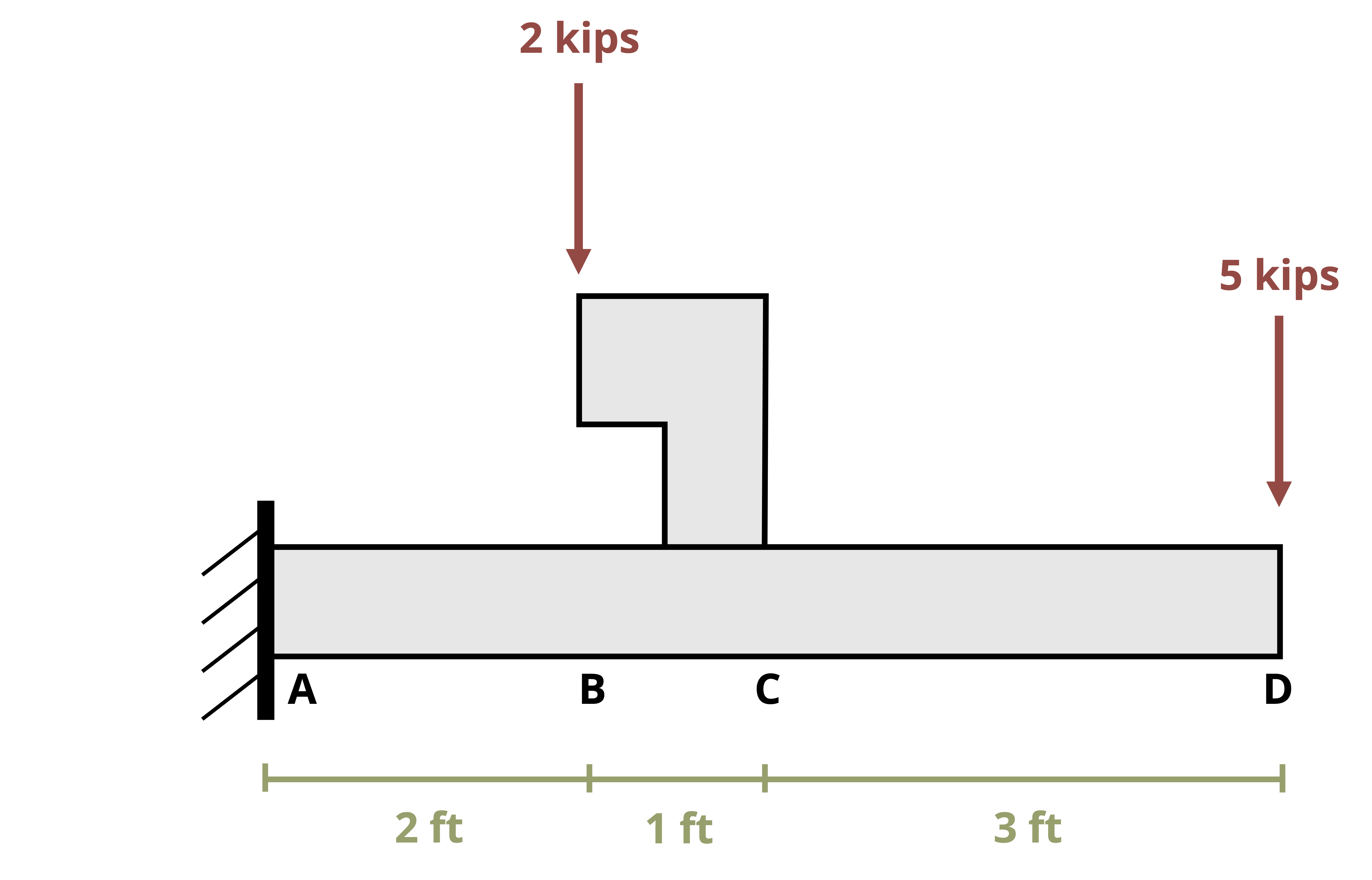
This beam differs a little from other examples in this chapter as the support is a fixed end and includes a force-couple system at point C. Nonetheless, the processes that have been presented here apply in this situation.
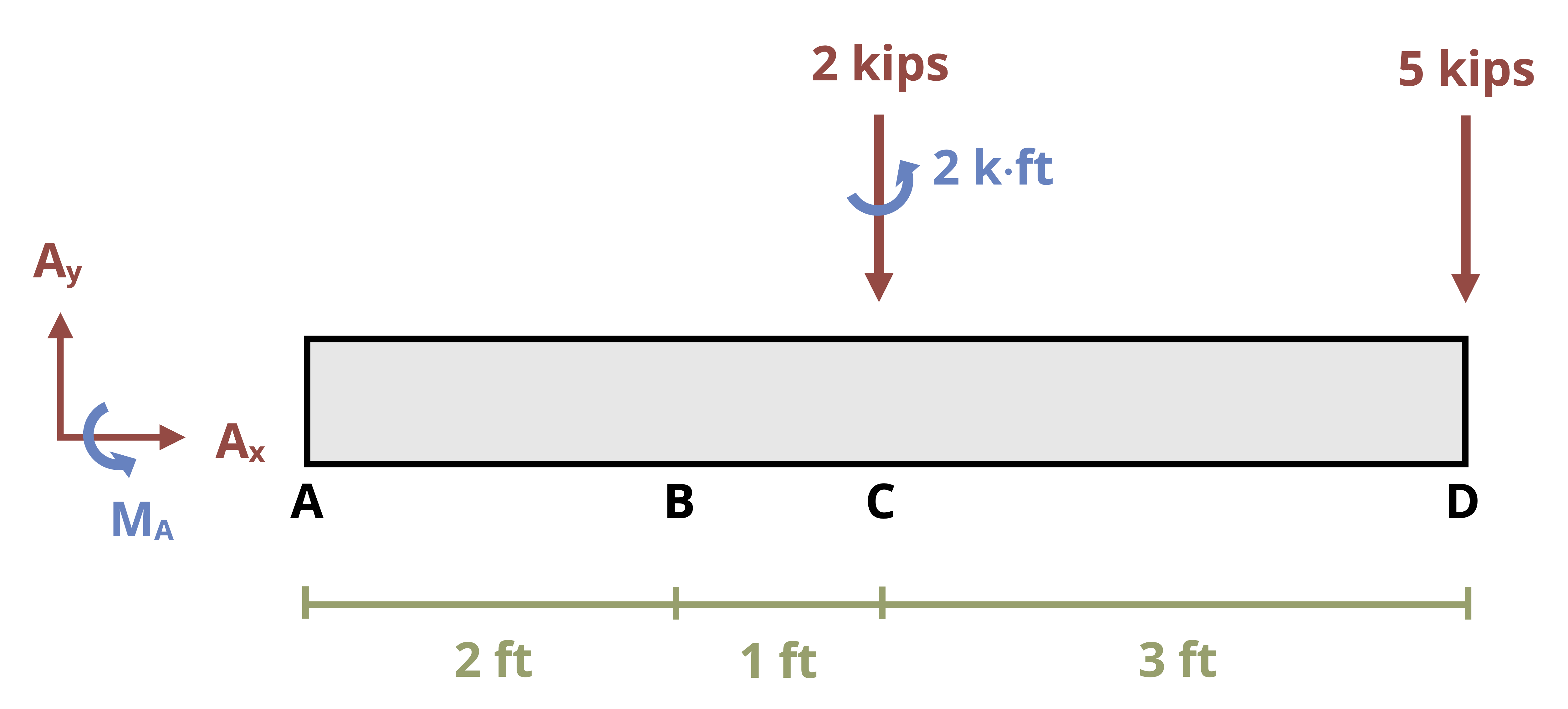
The first step is to draw an FBD of the beam, being sure to change the supports to the correct external reaction forces, as shown to the left. The 2 kips that acts on the arm at point B will cause a force on beam AD at the connection point, C. Additionally, a concentrated moment from this force also acts at point C. The magnitude of this concentrated moment is (2 kips)(1 ft) or 2 k·ft counterclockwise.
We then use static equilibrium equations to solve for the magnitude of the support reactions.
\[ \begin{aligned} &\sum F_x=A x=0 \\ &\sum F_y=A_y-2{~kips}-5{~kips}=0 \quad\rightarrow\quad A_y=7{~kips} \\ &\sum M_A = M_A + 2{~kip\cdot ft} - 2{~kips}(3{~ft}) - 5{~kips}(6{~ft})=0 \quad\rightarrow\quad M_A=34{~kip\cdot ft} \\ \end{aligned} \]
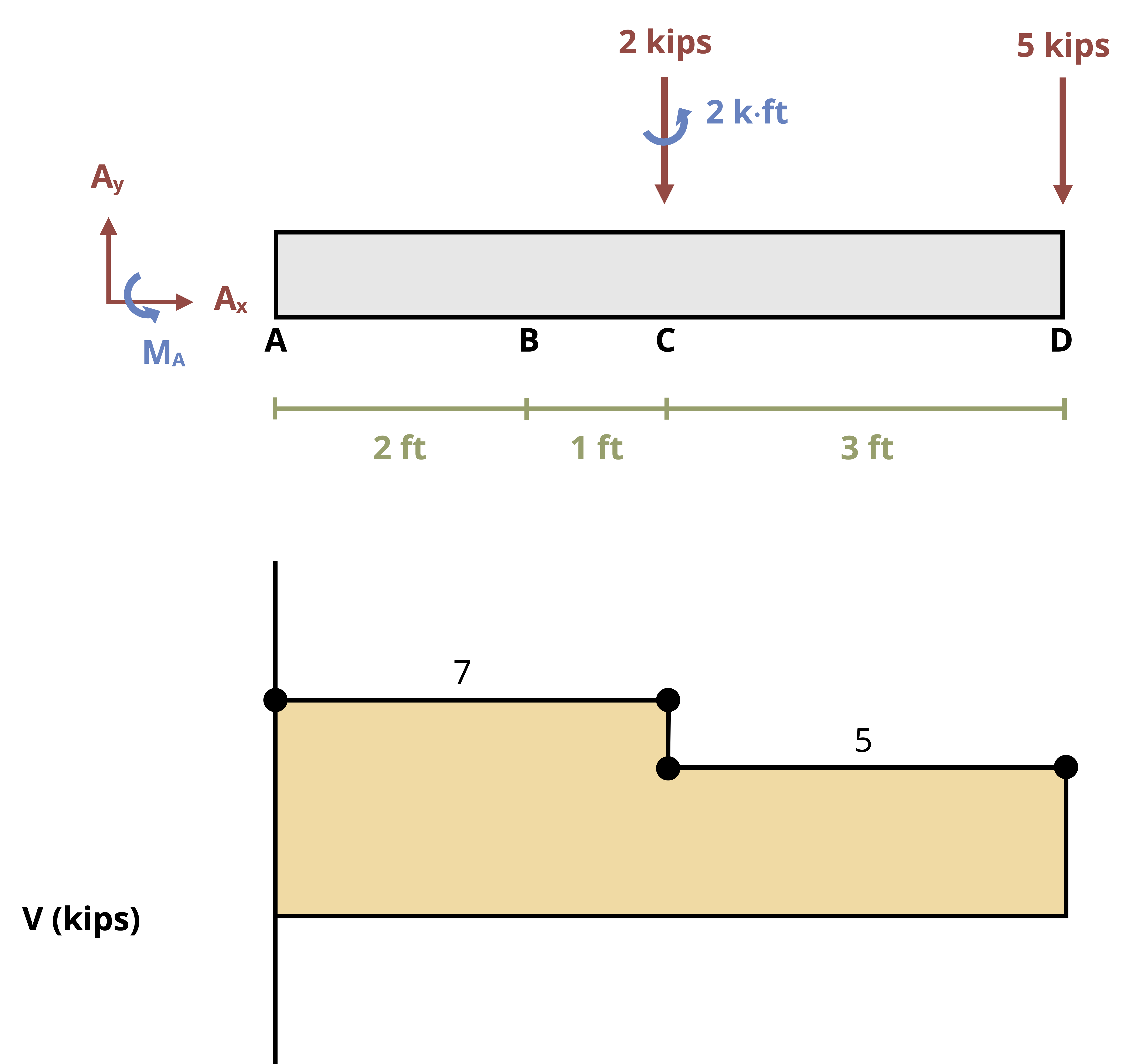
We can now build the shear diagram. Keep in mind that the concentrated moments (at points A and C) do not contribute to the shear diagram.
We start with the vertical reaction at point A. This is going up 7 kips. Then because no loads are on the beam between A and C, the shear diagram remains constant.
The concentrated force at point C is 2 kips down. So we subtract 2 kips from 7 kips. With no loads between points C and D, the shear diagram remains constant at 5 kips.
At point D there is a concentrated load of 5 kips down. This brings the shear diagram to a close at zero.
We next build the moment diagram with the combination of the area of the shear diagram and the concentrated moments.
We start from zero and go down 34 kip·ft since the reaction at A, MA, is counterclockwise.
Between A and B
Magnitude of the Change
Magnitude of the change encompasses the area under the curve. The height of the rectangle is 7 kips and the width is 3 ft, so the area is 21 kip·ft.
Direction of the Change
This area is on the positive side of the shear diagram, which indicates it will go up from A to C. We add the area from the internal moment at A (-34 + 21 = -13 kip·ft).
Shape of the Segment
The shear diagram is constant, so the moment diagram is linear with a slope of +7 kips/ft.
An applied concentrated moment of 2 kip·ft counterclockwise at point C creates a discontinuity in the moment diagram by dropping down 2 (-13 - 2 = -15 kip·ft).
Between C and D
Magnitude of the Change
Magnitude of the change encompasses the area under the curve. The height of the rectangle is 5 kips and the width is 3 ft, so the area is 15 kip·ft.
Direction of the Change
This area is on the positive side of the shear diagram, which indicates it will go up from C to D. Here we add the area from the internal moment at A (-15 + 15 = 0).
Shape of the Segment
The shear diagram is constant, so the moment diagram is linear with a slope of +5 kip/ft.
The final shear and moment diagram is in the figure to the left. Note that this cantilever structure with downward loads will bend concave down. This indicates that the entire beam will be in negative moment—which is also what our moment diagram indicates.
Summary
Click to expand
Shear and moment diagrams allow us to calculate and visualize the internal forces of beams. These internal forces are used to calculate stresses and deformations (covered in upcoming chapters). The general procedure for building the shear and moment diagrams is as follows:
- Sketch the beam, replacing support conditions with equivalent force(s).
- Find the support reactions using equilibrium.
- Use the method of equations or geometry or a combination to build the shear diagram directly below your beam sketch.
- Use the method of equations or geometry or a combination to build the moment diagram directly below your shear diagram.
- Ensure that your diagrams are labeled, including units, and that all pertinent values are indicated.
Relationship between load and shear:
\[ \Delta V=\Delta F \] \[ \underbrace{\Delta v}_{\substack{\text{change in} \\ \text{shear}}}=\int\underbrace{w d x}_{\substack{\text{area under} \\ \text {loading curve}}} \]
Relationship between shear and bending:
\[ d M=V d x \] \[ \underbrace{\Delta M}_{\text {Change in moment}}=\underbrace{\int V d x}_{\text {Area under shear diagram }} \]
References
Click to expand
Figures
All figures in this chapter were created by Kindred Grey in 2025 and released under a CC BY license, except for
- Figure 7.1: Examples of structural beams. A: Washington State Dept of Transportation. 2023. CC BY-NC-ND. https://flic.kr/p/2ojECo3. B: Government of Prince Edward Island. 2017. CC BY-NC-ND. https://flic.kr/p/R3NFRw. C: Jack E Boucher. 1985. Public domain. https://commons.wikimedia.org/wiki/File:FallingwaterCantilever570320cv.jpg.